Univariate Time Series using Facebook Prophet

A time series is a series of data points indexed in time order. Time series data can be stock prices, weather records, product sales, forex exchange, and health records. <!--more--> In investing, a time series model tracks the movement of stock prices over time. The model then predicts future stock prices based on previously historical/observed prices.

Time-series data can be univariate, bivariate, or multivariate. In this tutorial, we will be focusing on a univariate time series model. We will train the model using Facebook Prophet. This model will predict airline passengers.

Table of contents #

• Prerequisites
• Univariate vs Bivariate vs Multivariate datasets
• Getting started with Facebook Prophet
• Benefits of using Facebook Prophet
• Installing Facebook Prophet
• Airline passengers dataset
• Plotting the line chart
• Changing the column names
• Plotting an interactive line chart
• Building the model using Facebook Prophet
• Making future predictions
• Calling the predict method
• y vs yhat line chart
• Plot diagram
• Components of our forecasts
• Conclusion
• References

Prerequisites #

To follow along a reader should:

• Understand time series concepts.
• Understand time series decomposition in Python
• Know how to work with a time series dataset
• Know how to use Matplotlib library.

Univariate vs Bivariate vs Multivariate datasets #

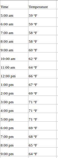
Univariate data #

It consists of only one variable that changes over time. Univariate data is simple because we are dealing with a single variable.

The image below shows an example of univariate data:

Image Source: Analyticsvidhya

Bivariate data #

It consists of two variables. The analysis of bivariate data involves finding the relationships between two variables.

The image below shows an example of bivariate data:

Image Source: GeeksforGeeks

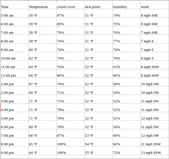
Multivariate data #

It consists of more than two variables. The analysis of multivariate data is more complicated. We have to find the relationships among all the variables.

The image below shows an example of multivariate data:

Image Source: Analyticsvidhya

Getting started with Facebook Prophet #

Facebook Prophet is an open-source library for forecasting time series data. It helps individuals and businesses analyze the market values and make future predictions.

It implements a procedure for forecasting time series data based on an additive model where non-linear trends are fit with yearly, weekly, and daily seasonality, plus holiday effects. It works best with time series with seasonal effects and several seasons of historical data.

It decomposes time series data into the following components:

Trend #

It is visible a pattern in data. It models non-periodic changes in the time series data. A trend shows the long-term movement in the dataset. A trend can be upward (uptrend), downward (downtrend), or constant (horizontal). Trends usually happen for some time and then disappear.

The image below shows the three types of trends.

Image Source: Medium

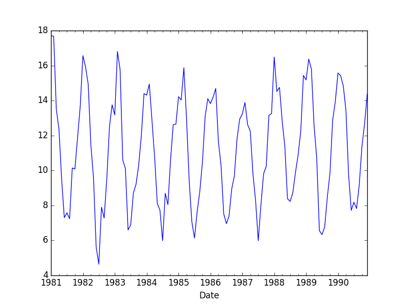
Seasonality #

It is due to periodic changes like daily, weekly, or yearly seasonality.

The image below shows a seasonality component.

Image Source: Machine Learning Mastery

Holiday effect #

It is the recurring days and events in a time series dataset. It involves the occurrence of popular holidays such as Christmas and others.

Benefits of using Facebook Prophet #

The following are the benefits of using Facebook Prophet in time series modeling.

• It is automatic and fast. It saves time for manual time series analysis and decomposition.

• It produces reliable and accurate models.

• It can handle missing values and outliers. It imputes the missing values to ensure we have a complete dataset. It also removes data points that deviate from the general dataset observations.

• It can handle seasonality and holiday effects. It handles the spikes in the dataset and include them in model training.

• It produces a tunable model. It produces models that we fine-tune to improve accuracy when forecasting.

Installing Facebook Prophet #

To install Facebook Prophet, use this command:

!pip install fbprophet

Airline passengers dataset #

We will use the airline passengers dataset to train the model. The dataset shows the airline passengers recorded monthly from 1949-01-01 to 1960-12-01. It has only a one-time dependant variable. To download the dataset, use this link

We will read the dataset using Pandas.

import pandas as pd

We read the dataset using this code:

df=pd.read_csv('/content/airline_passengers.csv')

To see the first five rows of our dataset, use this code:

df.head()

It produces the following output:

It has two columns, Month and Thousands of Passengers. The model will use the Thousands of Passengers column as the input variable. Thousands of Passengers is the one variable in the dataset that changes over time.

To see the last five rows of our dataset, use this code:

df.tail()

The output:

From the image above, the last column has null values. We will drop this column.

df.drop(144,axis=0,inplace=True)

Plotting the line chart #

We will plot the line chart using Matplotlib.

import matplotlib.pyplot as plt
%matplotlib inline

To plot the line chart, use this code:

df.plot()

The line chart:

From the image above, the dataset is on an uptrend. The number of airline passengers has been increasing over time.

Changing the column names #

Facebook Prophets expects an input Data Frame with two columns named ds and y. ds column contains the dates/timestamp of the time series . y has the times series values (data points).

df.columns = ['ds','y']

To see the dataset, use this code:

df.head()

The output:

Plotting an interactive line chart #

We will use the Plotly Express library to plot a more interactive line chart.

import plotly.express as px

To plot the line chart, use this code:

fig = px.line(df, x='ds', y='y', title='Airline Passengers')

fig.update_xaxes(
    rangeslider_visible=True,
    rangeselector=dict(
        buttons=list([
            dict(step="all")
        ])
    )
)
fig.show()

From the code above, ds is the x-axis and y the y-axis. Airline Passengers is the title of the line chart. rangeslider_visible will enable us to zoom the line chart. rangeselector will select some of the data points on the line chart.

The line chart output:

Converting the 'ds' column #

We need to convert the ds column to the DateTime format. It will enable us to perform time-series operations and analysis on this column. We will use the Python Datetime module.

from datetime import datetime

Use this code to convert the ds column:

df['ds'] = pd.to_datetime(df['ds'])

Use this code to view the dataset:

df.head()

The output:

To see the last five rows of our dataset, use this code:

df.tail()

The output:

Building the model using Facebook Prophet #

We import Facebook Prophet using this code:

from fbprophet import Prophet

Initializing the model #

Use the code below:

model=Prophet()

The Prophet class has initialized the model.

Calling the fit method #

We call the fit method and pass the Data Frame as an input. The fit enables the model to find patterns in the data. It will aid the model in forecasting future values.

model.fit(df)

Making future predictions #

The process above trains the model. We will use the model to forecast the airline passengers for the next 1000 days (1961-01-01 to 1963-08-28). We will provide the model with a new future Data Frame. It contains the number of days the model forecasts/predicts.

We use this code:

future_dates=model.make_future_dataframe(periods=1000, freq='M')

Use this code to check the last five rows:

future_dates.tail()

The output is shown below:

Calling the predict method #

We call the predict method and pass the future_dates as an input.

prediction=model.predict(future_dates)

Use this code to see the last five rows of the prediction results:

prediction[['ds', 'yhat', 'yhat_lower', 'yhat_upper']].tail()

The prediction Data Frame has the following columns:

• ds: It contains the datestamp of the forecasted values. It holds the timestamp of 1000 days.
• yhat: It contains the prediction/forecast values of the time series model.
• yhat_lower: It contains the lower bound of the prediction/forecast values.
• yhat_upper: It contains the upper bound of the prediction/forecast values.

The prediction values:

Use this code to see the first five rows of the prediction results:

prediction.head()

The output:

'y' vs 'yhat' line chart #

Use this code to plot the line chart:

pd.concat([df.set_index('ds')['y'],prediction.set_index('ds')['yhat']],axis=1).plot()

The code produces the following line chart:

From the output above:

• The blue line shows the actual values (y).
• The orange line shows the predicted values (yhat).
• The chart also shows the forecast values for the next 1000 days.

We can also plot a diagram to show the y, yhat, yhat_lower, and the yhat_upper values.

Plot diagram #

Use this code:

model.plot(prediction)

The output:

From the output above:

• The shaded light blue region shows the lower and upper bound values. This region contains the yhat_upper and yhat_lower values.
• The black dots are the actual time series values (y).
• The blue line shows the predicted values (yhat).
• The chart also shows the forecast values for the next 1000 days.

We can also use Facebook Prophet to plot the components of our forecasts.

Components of our forecast #

Use this code to plot the components:

model.plot_components(prediction)

The output:

The output above shows the trend and yearly seasonality components. The above plots provide insights. The first plot shows a linear increase in passengers from 1949 to 1964. The second plot shows that most traffic occurs during the holiday months of July and August.

Conclusion #

In this tutorial, we have learned how to build a univariate time series model using Facebook Prophet. We discussed the different types of time-series datasets. We were able to differentiate univariate, bivariate, and multivariate datasets. We explored Facebook Prophet and how it decomposes time-series datasets.

We trained a time series model which forecasts airline passengers. Finally, we used Facebook Prophet to plot the components of our forecasts.

To access the Google Colab notebook for this tutorial, click here.

References #

• Time Series Decomposition in Python
• Introduction to Time Series
• Facebook Prophet Github
• Univariate vs Bivariate vs Multivariate datasets
• Introduction to Time Series with Facebook Prophet

---

Peer Review Contributions by: Wilkister Mumbi