

Multi-Class Text Classification with PySpark

PySpark is a python API written as a wrapper around the Apache Spark framework. Apache Spark is an open-source Python framework used for processing big data and data mining.
Apache Spark is best known for its speed when it comes to data processing and its ease of use. It has a high computation power, that's why it's best suited for big data. It supports popular libraries such as Pandas, Scikit-Learn and NumPy used in data preparation and model building.
We will use PySpark to build our multi-class text classification model. This involves classifying the subject category given the course title. We have various subjects in our dataset that can be assigned, specific classes.
Table of contents
- Prerequisites
- Introduction
- PySpark Installation
- Creating SparkContext and SparkSession
- Initializing the TextClassifier app
- Loading Dataset
- Selecting the needed columns
- Checking for missing values
- Feature Engineering
- Pipeline stages
- Splitting our dataset
- Building the pipeline
- Building model
- Model evaluation
- Making a single prediction
- Conclusion
- References
Prerequisites
A reader must have:
- A good understanding of Python.
- Anaconda installed on your machine.
- A good knowledge of Jupyter Notebook.
- An understanding of machine learning modeling.
- Downloaded the Udemy dataset.
NOTE: To follow along easily, use Jupyter Notebook to build your text classification model.
Introduction
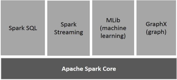
Pyspark uses the Spark API in data processing and model building. Spark API consists of the following libraries:
Spark SQL
This is the structured query language used in data processing. It's used to query the datasets in exploring the data used in model building.
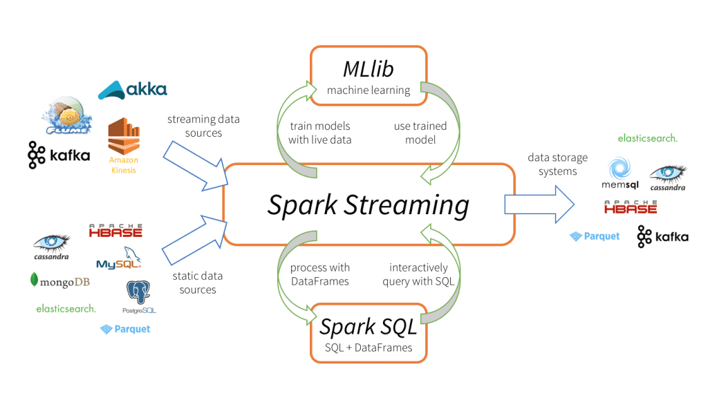
Spark Streaming
This library allows the processing and analysis of real-time data from various sources such as Flume, Kafka, and Amazon Kinesis.
The image below shows the components of spark streaming:

MLib
Mlib contains a uniform set of high-level APIs used in model creation. It helps to train our model and find the best algorithm.
Spark Core
This is the root of the Spark API. It's involved with the core functionalities such as basic I/O functionalities, task scheduling, and memory management.
GraphX
It is used in the plotting of graphs for Spark computations.
The image below shows components of the Spark API:

Pyspark supports two data structures that are used during data processing and machine learning building:
Resilient Distributed Dataset (RDD)
This is a distributed collection of data spread and distributed across multiple machines in a cluster.
RDD is best described in three ways:
- Resilient: Fault-tolerant and can rebuild itself if a failure occurs.
- Distributed: Data is distributed among the multiple nodes in a cluster.
- Dataset: Collection of partitioned data with values.
Dataframe
Dataframe in PySpark is the distributed collection of structured or semi-structured data. This data in Dataframe is stored in rows under named columns. It is similar to relational database tables or excel sheets.
These two define the nature of the dataset that we will be using when building a model.
API's used for machine learning
There are two APIs that are used for machine learning:
PySpark.ML
It contains a high-level API built on top of data frames used in building machine learning models. It has easy-to-use machine learning pipelines used to automate the machine learning workflow.
PySpark.MLib
It contains a high-level API built on top of RDD that is used in building machine learning models. It consists of learning algorithms for regression, classification, clustering, and collaborative filtering.
In this tutorial, we will use the PySpark.ML API in building our multi-class text classification model.
NOTE: We are using
PySpark.ML APIin building our model becausePySpark.MLibis deprecated and will be removed in the next PySpark release.
To learn more about the components of PySpark and how it’s useful in processing big data, click here.
PySpark Installation
We install PySpark by creating a virtual environment that keeps all the dependencies required for our project. Before we install PySpark, we need to have pipenv in our machine and we install it using the following command:
pip install pipenv
We can now install PySpark using this command:
pipenv install pyspark
Since we are using Jupyter Notebook in this tutorial, we install jupyterlab using the following command:
pipenv install jupyterlab
To launch PySpark, use this command:
pipenv run pyspark
The above command will launch PySpark.
Let's now activate the virtual environment that we have created.
pipenv shell
To launch our notebook, use this command:
pipenv run jupyter lab
This command will launch the notebook. From here, we can start working on our model.
Creating SparkContext and SparkSession
In this tutorial, we will be building a multi-class text classification model. The model can predict the subject category given a course title or text. We will use the Udemy dataset in building our model.
Let's import our machine learning packages:
import SparkContext from pyspark
SparkContext creates an entry point of our application and creates a connection between the different clusters in our machine allowing communication between them.
'SparkContext' will also give a user interface that will show us all the jobs running. The master option specifies the master URL for our distributed cluster which will run locally. We also specify the number of threads to 2. This allows our program to run 2 threads concurrently. It reduces the failure of our program.
sc = SparkContext(master="local[2]")
To launch the Spark dashboard use the following command:
sc
Note that the Spark Dashboard will run in the background.
The output is as shown below:
Spark UI

Version
v3.0.2
Master
local[2]
AppName
pyspark-shell
In the above output, the Spark UI is a link that opens the Spark dashboard in localhost: http://192.168.0.6:4040/, which will be running in the background. When one clicks the link it will open a Spark dashboard that shows the available jobs running on our machine. Currently, we have no running jobs as shown:

Creating SparkSession
By creating SparkSession, it enables us to interact with the different Spark functionalities. The functionalities include data analysis and creating our text classification model.
import SparkSession from pyspark.sql
In the above code command, we create an entry point to programming Spark. A SparkSession creates our DataFrame, registers DataFrame as tables, execute SQL over tables, cache tables, and read files.
Initializing the TextClassifier app
Using the imported SparkSession we can now initialize our app.
spark = SparkSession.builder.appName("TextClassifierApp").getOrCreate()
We use the builder.appName() method to give a name to our app.
After initializing our app, we can now view our launched UI to see the running jobs. The running jobs are shown below:


Loading dataset
We use the Udemy dataset that contains all the courses offered by Udemy. The dataset contains the course title and subject they belong.

To get the CSV file of this dataset, click here.
After you have downloaded the dataset using the link above, we can now load our dataset into our machine using the following snippet:
df = spark.read.csv("udemy_dataset.csv",header=True,inferSchema=True)
To show the structure of our dataset, use the following command:
df.show()

To see the available columns in our dataset, we use the df.column command as shown:
df.columns
Output:
['_c0',
 'course_id',
 'course_title',
 'url',
 'is_paid',
 'price',
 'num_subscribers',
 'num_reviews',
 'num_lectures',
 'level',
 'content_duration',
 'published_timestamp',
 'subject',
 'clean_course_title']

In this tutorial, we will use the course_title and subject columns in building our model.
Selecting the needed columns
We select the course_title and subject columns. These are the columns we will use in building our model.
df.select('course_title','subject').show()
The output of the available course_title and subject in the dataset is shown.
+--------------------+----------------+
|        course_title|         subject|
+--------------------+----------------+
|Ultimate Investme...|Business Finance|
|Complete GST Cour...|Business Finance|
|Financial Modeling...|Business Finance|
|Beginner to Pro -...|Business Finance|
|How To Maximize Y...|Business Finance|
|Trading Penny Sto...|Business Finance|
|Investing And Tra...|Business Finance|
|Trading Stock Cha...|Business Finance|
|Options Trading 3...|Business Finance|
|The Only Investme...|Business Finance|
|Forex Trading Sec...|Business Finance|
|Trading Options W...|Business Finance|
|Financial Managem...|Business Finance|
|Forex Trading Cou...|Business Finance|
|Python Algo Trading...|Business Finance|
|Short Selling: Le...|Business Finance|
|Basic Technical A...|Business Finance|
|The Complete Char...|Business Finance|
|7 Deadly Mistakes...|Business Finance|
|Financial Stateme...|Business Finance|
+--------------------+----------------+
Note: This only shows the top 20 rows.
Let's save our selected columns in the df variable.
df = df.select('course_title','subject')
Checking for missing values
We need to check for any missing values in our dataset. This ensures that we have a well-formatted dataset that trains our model.
df.toPandas()['subject'].isnull().sum()
We use the toPandas() method to check for missing values in our subject column and drop the missing values.
df = df.dropna(subset=('subject'))
This will drop all the missing values in our subject column.
Feature engineering
Feature engineering is the process of getting the relevant features and characteristics from raw data. We extract various characteristics from our Udemy dataset that will act as inputs into our machine. The features will be used in making predictions.
Machine learning algorithms do not understand texts so we have to convert them into numeric values during this stage.
We import all the packages required for feature engineering:
import pyspark.ml.feature
To list all the available methods, run this command:
dir(pyspark.ml.feature)
These features are in form of an extractor, vectorizer, and tokenizer.
- Tokenizer
It involves splitting a sentence into smaller words. This tutorial will convert the input text in our dataset into word tokens that our machine can understand. For a detailed understanding of Tokenizer click here.
- CountVectorizer
It is a great tool in machine learning that converts our given text into vectors of numeric numbers. Machines understand numeric values easily rather than text. For a detailed understanding about CountVectorizer click here.
- Extractor
This is the process of extract various characteristics and features from our dataset. This enables our model to understand patterns during predictive analysis. To automate these processes, we will use a machine learning pipeline. This will simplify the machine learning workflow.
Pipeline stages
We will use the pipeline to automate the process of machine learning from the process of feature engineering to model building.
The pipeline stages are categorized into two:

- Transformers
This includes different methods that take data and fit them into the data or feature.
Transformers involves the following stages:
Tokenizer
It converts the input text and converts it into word tokens. These word tokens are short phrases that act as inputs into our model.
For detailed information about Tokenizer click here.
StopWordsRemover
It extracts all the stop words available in our dataset. Stop words are a set of words that are used in a given sentence frequently. These words may be biased when building the classifier.
For a detailed information about StopWordsRemover click here.
CountVectorizer
It converts from text to vectors of numbers. Numbers are understood by the machine easily rather than text.
For a detailed information about CountVectorizer click here.
Inverse Document Frequency(IDF)
It's a statistical measure that indicates how important a word is relative to other documents in a collection of documents. This creates a relation between different words in a document.
If a word appears frequently in a given document and also appears frequently in other documents, it shows that it has little predictive power towards classification. The more the word is rare in given documents, the more it has value in predictive analysis.
For a detailed understanding of IDF click here.
- Estimators
An estimator takes data as input, fits the model into the data, and produces a model we can use to make predictions.
LogisticRegression
This is the algorithm that we will use in building our model. It's a statistical analysis method used to predict an output based on prior pattern recognition and analysis.
We shall have five pipeline stages: Tokenizer, StopWordsRemover, CountVectorizer, Inverse Document Frequency(IDF), and LogisticRegression.
Let's import the packages required to initialize the pipeline stages.
from pyspark.ml.feature import Tokenizer,StopWordsRemover,CountVectorizer,IDF
We also need to import StringIndexer.
StringIndexer is used to add labels to our dataset. Labels are the output we intend to predict.
from pyspark.ml.feature import StringIndexer
Initializing the pipeline stages
We need to initialize the pipeline stages. As mentioned earlier our pipeline is categorized into two: transformers and estimators.
In this section, we initialize the 4 stages found in the transformers category. Later we will initialize the last stage found in the estimators category.
The transformers category stages are as shown:
tokenizer.stopwords_remover.vectorizer.idf.
The pipeline stages are sequential, the first stage has a column named course_title which is transformed into mytokens as the output column. The columns are further transformed until we reach the vectorizedFeatures after the four pipeline stages.
vectorizedFeatures will now become the input of the last pipeline stage which is LogisticRegression. The last stage is where we build our model.
This is a sequential process starting from the tokenizer stage to the idf stage as shown below:
tokenizer = Tokenizer(inputCol='course_title',outputCol='mytokens')
stopwords_remover = StopWordsRemover(inputCol='mytokens',outputCol='filtered_tokens')
vectorizer = CountVectorizer(inputCol='filtered_tokens',outputCol='rawFeatures')
idf = IDF(inputCol='rawFeatures',outputCol='vectorizedFeatures')
This will create the pipeline stages.
Adding labels
labelEncoder = StringIndexer(inputCol='subject',outputCol='label').fit(df)
We add labels into our subject column to be used when predicting the type of subject. This helps our model to know what it intends to predict. We use the StringIndexer function to add our labels.
To see how the different subjects are labeled, use the following code:
labelEncoder.transform(df).show(5)
The output is as shown:
labelEncoder.transform(df).show(5)
+--------------------+----------------+-----+
|        course_title|         subject|label|
+--------------------+----------------+-----+
|Ultimate Investme...|Business Finance|  1.0|
|Complete GST Cour...|Business Finance|  1.0|
|Financial Modeling...|Business Finance|  1.0|
|Beginner to Pro -...|Business Finance|  1.0|
|How To Maximize Y...|Business Finance|  1.0|
+--------------------+----------------+-----+
Note: This only shows the top 5 rows.
Dictionary of all labels
We have to assign numeric values to the subject categories available in our dataset for easy predictions.
label_dict = {'Web Development':0.0,
 'Business Finance':1.0,
 'Musical Instruments':2.0,
 'Graphic Design':3.0}
As shown, Web Development is assigned 0.0, Business Finance assigned 1.0, Musical Instruments assigned 2.0, and Graphic Design assigned 3.0.
We add these labels into our dataset as shown:
df = labelEncoder.transform(df)
We use the transform() method to add the labels to the respective subject categories.
The output below shows that our data is labeled:
+--------------------+--------------------+-----+
|        course_title|             subject|label|
+--------------------+--------------------+-----+
|1 Piano Hand Coo...| Musical Instruments|  2.0|
|10 Hand Coordina...| Musical Instruments|  2.0|
|4 Piano Hand Coo...| Musical Instruments|  2.0|
|5  Piano Hand Co...| Musical Instruments|  2.0|
|6 Piano Hand Coo...| Musical Instruments|  2.0|
|Geometry Of Chan...|    Business Finance|  1.0|
|1 - Concepts of S...|   Business Finance|  1.0|
|          1 Hour CSS|    Web Development|  0.0|
|1. Principles of ...|   Business Finance|  1.0|
|10 Numbers Every ...|   Business Finance|  1.0|
|10.  Bonds and Bo...|   Business Finance|  1.0|
|101 Blues riffs -...|Musical Instruments|  2.0|
|15 Mandamientos p...|   Business Finance|  1.0|
|17 Complete JavaS...|    Web Development|  0.0|
|188% Profit in 1Y...|   Business Finance|  1.0|
|2 Easy Steps To I...|   Business Finance|  1.0|
|3 step formula fo...|Musical Instruments|  2.0|
|30 Day Guitar Jum...|Musical Instruments|  2.0|
|3DS MAX - Learn 3...|     Graphic Design|  3.0|
+--------------------+--------------------+-----+
Note: This only shows the top 20 rows.
Splitting our dataset
We split our dataset into train set and test set. This data is used as the input in the last pipeline stage.
The last stage involves building our model using the LogisticRegression algorithm.
(trainDF,testDF) = df.randomSplit((0.7,0.3),seed=42)
70% of our dataset will be used for training and 30% for testing.
Importing LogisticRegression
We import the LogisticRegression algorithm which we will use in building our model to perform classification.
from pyspark.ml.classification import LogisticRegression
Creating estimator
An estimator is a function that takes data as input, fits the data, and creates a model used to make predictions.
lr = LogisticRegression(featuresCol='vectorizedFeatures',labelCol='label')
The IDF stage inputs vectorizedFeatures into this stage of the pipeline. vectorizedFeatures will be used as the input column used by the LogisticRegression algorithm to build our model and our target label will be the label column.
We have initialized all five pipeline stages. We can start building the pipeline to perform these tasks.
Building the pipeline
Let's import the Pipeline() method that we'll use to build our model.
import Pipeline from pyspark.ml
Fitting the five stages
We add the initialized 5 stages into the Pipeline() method.
pipeline = Pipeline(stages=[tokenizer,stopwords_remover,vectorizer,idf,lr])
Building model
We build our model by fitting our model into our training dataset by using the fit() method and passing the trainDF as our parameter.
Let's initialize our model pipeline as lr_model.
lr_model = pipeline.fit(trainDF)
Testing model
We test our model using the test dataset to see if it can classify the course title and assign the right subject.
predictions = lr_model.transform(testDF)
To see if our model was able to do the right classification, use the following command:
predictions.show()

To get all the available columns use this command.
predictions.columns
The output of the columns is as shown.
['course_title',
 'subject',
 'label',
 'mytokens',
 'filtered_tokens',
 'rawFeatures',
 'vectorizedFeatures',
 'rawPrediction',
 'probability',
 'prediction']
From the above columns, we select the necessary columns used for predictions and view the first 10 rows.
predictions.select('rawPrediction','probability','subject','label','prediction').show(10)
The output is as shown:
+--------------------+--------------------+-------------------+-----+----------+
|       rawPrediction|         probability|            subject|label|prediction|
+--------------------+--------------------+-------------------+-----+----------+
|[8.22575678849003...|[0.86083740538013...|Musical Instruments|  2.0|       0.0|
|[-1.5816511969981...|[6.40379189870091...|Musical Instruments|  2.0|       2.0|
|[0.38747123626564...|[1.29430064456987...|Musical Instruments|  2.0|       2.0|
|[-2.0540053505355...|[3.67476794956146...|   Business Finance|  1.0|       1.0|
|[24.7266193282529...|[0.99999999908079...|    Web Development|  0.0|       0.0|
|[22.2213462251437...|[0.99999999175336...|    Web Development|  0.0|       0.0|
|[20.1005546377385...|[0.99999995838555...|    Web Development|  0.0|       0.0|
|[-5.9910327938499...|[2.64083766762944...|Musical Instruments|  2.0|       2.0|
|[-19.729920863390...|[4.16984026967754...|     Graphic Design|  3.0|       3.0|
|[-2.6725325296694...|[9.29048167255554...|Musical Instruments|  2.0|       2.0|
+--------------------+--------------------+-------------------+-----+----------+
Note: This is only showing the top 10 rows.
From the above output, we can see that our model can accurately make predictions. The label columns match with the prediction columns.
Model evaluation
This is checking the model accuracy so that we can know how well we trained our model.
Let's import the MulticlassClassificationEvaluator. We'll use it to evaluate our model and calculate the accuracy score.
from pyspark.ml.evaluation import MulticlassClassificationEvaluator
The MulticlassClassificationEvaluator uses the label, column and prediction columns to calculate the accuracy. If the two-column matches, it increases the accuracy score of our model.
evaluator = MulticlassClassificationEvaluator(labelCol='label',predictionCol='prediction',metricName='accuracy')
accuracy = evaluator.evaluate(predictions)
To get the accuracy, run the following command:
accuracy
The output is shown:
0.9163498098859315
This shows that our model is 91.635% accurate.
Making a single prediction
We use our trained model to make a single prediction. We input a text into our model and see if our model can classify the right subject.
Single predictions expose our model to a new set of data that is not available in the training set or the testing set. This makes sure that our model makes new predictions on its own under a new environment.
To perform a single prediction, we prepare our sample input as a string.
We use the StringType() function.
from pyspark.sql.types import StringType
Create a sample data frame made up of the course_title column.
ex1 = spark.createDataFrame([
    ("Building Machine Learning Apps with Python and PySpark",StringType())
],
["course_title"]

)
Let's output our data frame without truncating.
ex1.show(truncate=False)
After we formatting our input string, now let's make a prediction.
pred_ex1 = lr_model.transform(ex1)
To show the output, use the following command:
pred_ex1.show()
Output:

Get all the available columns.
pred_ex1.columns
The output is as shown.
['course_title',
 '_2',
 'mytokens',
 'filtered_tokens',
 'rawFeatures',
 'vectorizedFeatures',
 'rawPrediction',
 'probability',
 'prediction']
From the above columns, let's select the necessary columns that give the prediction results.
pred_ex1.select('course_title','rawPrediction','probability','prediction').show()
Output:
+--------------------+--------------------+--------------------+----------+
|        course_title|       rawPrediction|         probability|prediction|
+--------------------+--------------------+--------------------+----------+
|Building Machine ...|[14.6893212262828...|[0.99999805300087...|       0.0|
+--------------------+--------------------+--------------------+----------+
The prediction is 0.0 which is web development according to our created label dictionary.
To see our label dictionary use the following command.
label_dict
The output of the label dictionary is as shown.
{'Web Development': 0.0,
 'Business Finance': 1.0,
 'Musical Instruments': 2.0,
 'Graphic Design': 3.0}
This shows that our model can accurately classify the given text into the right subject with an accuracy of 91.63498.
Conclusion
In the tutorial, we have learned about multi-class text classification with PySpark. We started with PySpark basics, learned the core components of PySpark used for Big Data processing. This gave us a good foundation and a good understanding of PySpark.
From here we then started preparing our dataset by removing missing values. We used the Udemy dataset to build our model.
We then followed the stages in the machine learning workflow. We started with feature engineering then applied the pipeline approach to automate certain workflows. Pipeline makes the process of building a machine learning model easier. After following all the pipeline stages, we ended up with a machine learning model.
Finally, we used this model to make predictions, this is the goal of any machine learning model. If a model can accurately make predictions, the better the model. Using these steps, a reader should comfortably build a multi-class text classification with PySpark.
Further reading
References
- Code implementation for this tutorial
- Introduction to PySpark
- PySpark Tutorial
- PySpark Components
- PySpark Documentation
- PySpark Basics
- Getting started with PySpark
Peer Review Contributions by: Willies Ogola


