

Dropout Regularization to Handle Overfitting in Deep Learning Models

Overfitting and underfitting are common problems in machine learning. Overfitting happens when a model perfectly learns during training but performs poorly during testing. The model will have a higher accuracy score on the training dataset but a lower accuracy score on the testing.
Underfitting occurs when the model can neither learn from the training data nor make predictions using a testing dataset. This model underperforms both in training and in testing. This model is too simple to learn anything.
Overfitting problem is more common than underfitting. We have many techniques that can handle overfitting such as cross-validation, data augmentation, feature selection, early stopping, and dropout regularization. We will focus on the dropout regularization technique.
In this tutorial, we will start by building a deep learning model using TensorFlow. We will then use the dropout regularization technique to handle overfitting. This will ensure that we have a model that has a good performance on both the training dataset and the testing dataset.
Table of contents
- Prerequisites
- Getting-started-with-dropout-regularization
- Exploring the dataset
- Dataset splitting
- Model without dropout regularization
- Initializing the sequential model
- Model compiling
- Model fitting
- Accuracy score using the testing dataset
- Model with dropout regularization
- Using testing dataset
- Conclusion
- References
Prerequisites
For a reader to follow this tutorial easily, he should:
- Know how to build deep learning models.
- Understand Pandas and Numpy for data analysis and manipulation.
- Know how to use TensorFlow and Keras in building neural networks.
- Use Google Colab notebook when building the neural network model.
Getting started with dropout regularization
Dropout regularization is a technique that randomly drops a number of neurons in a neural network during model training.
This means the contribution of the dropped neurons is temporally removed and they do not have an impact on the model's performance.
The image below shows how dropout regularization works:

In the image above, the neural network on the left shows an original neural network where all neurons are activated and working.
On the right, the red neurons have been removed from the neural network. Therefore, red neurons will not be considered during model training.
We will implement this concept practically using TensorFlow.
How will dropout help with overfitting?
Dropout regularization will ensure the following:
- The neurons can't rely on one input because it might be dropped out at random. This reduces bias due to over-relying on one input, bias is a major cause of overfitting.
- Neurons will not learn redundant details of inputs. This ensures only important information is stored by the neurons. This enables the neural network to gain useful knowledge which it uses to make predictions.
We will start by building a model without applying dropout regularization. Before we begin, let's explore the dataset we will use to build the model.
Exploring the dataset
The dataset used is the Sonar dataset. The dataset is used for the classification of sonar signals using a neural network. The model predicts if sonar signals are bounced off a metal surface or a rock surface.
To download the CSV file, click here.
To load the dataset, we use Pandas and Numpy. These are useful Python packages used for dataset manipulation and analysis.
import numpy as np
import pandas as pd
Let's load the dataset:
df = pd.read_csv("./sonar_dataset.csv", header=None)
To view our dataset, use this code:
print(df.sample(5))
The output of 5 data samples is shown below:

From the image above, the dataset has a total of 61 columns labeled from 0. The first 60 columns are the input columns for the model, the last column (60th) is the output column. The last column is either labeled R or M representing Rock and Metal respectively.
In our dataset, we have to create an X variable and a y variable. The X variable represents the input columns while the y variable represents the output/target column. We create our X variable and y variable as follows:
X = df.drop(60, axis=1)
y = df[60]
From the code above, the X variable holds values of the first 60 columns and the y variable is the last column (60th).
The last column is either labeled R or M, but we need to convert it to a number format. It should be either 0 or 1. We will be representing 1 for R, and 0 for M.
Machine learning models work well with numbers, unlike text which is a major problem to these models. To convert text to numbers we will use the get_dummies method which is a Pandas method.
y = pd.get_dummies(y, drop_first=True)
To view the converted column, run this code:
print(y.sample(5))
The output will give 5 data samples as shown below:

The next step is to split our dataset.
Dataset splitting
In this stage, we split the dataset into two sets. The first set will be used for training and the second set will be used for testing.
from sklearn.model_selection import train_test_split
X_train, X_test, y_train, y_test = train_test_split(X, y, test_size=0.25, random_state=1)
From the code above, we have imported train_test_split for dataset splitting.
We split our dataset using a test_size=0.25. This ensures that 75% of the dataset will be used for training and 25% will be used for testing.
After splitting the dataset, the next step is to first build the model without dropout regularization. In the later section, we will build the same model with dropout regularization.
Model without dropout regularization
Let's import the important libraries we will use to build our neural network.
import tensorflow as tf
from tensorflow import keras
We will use both TensorFlow and Keras for building our neural network. TensorFlow will run our backend when training the neural network. Keras will create the input, hidden and output layers of our neural network.
In TensorFlow, we have two types of models:
- Sequential model.
- Functional model.
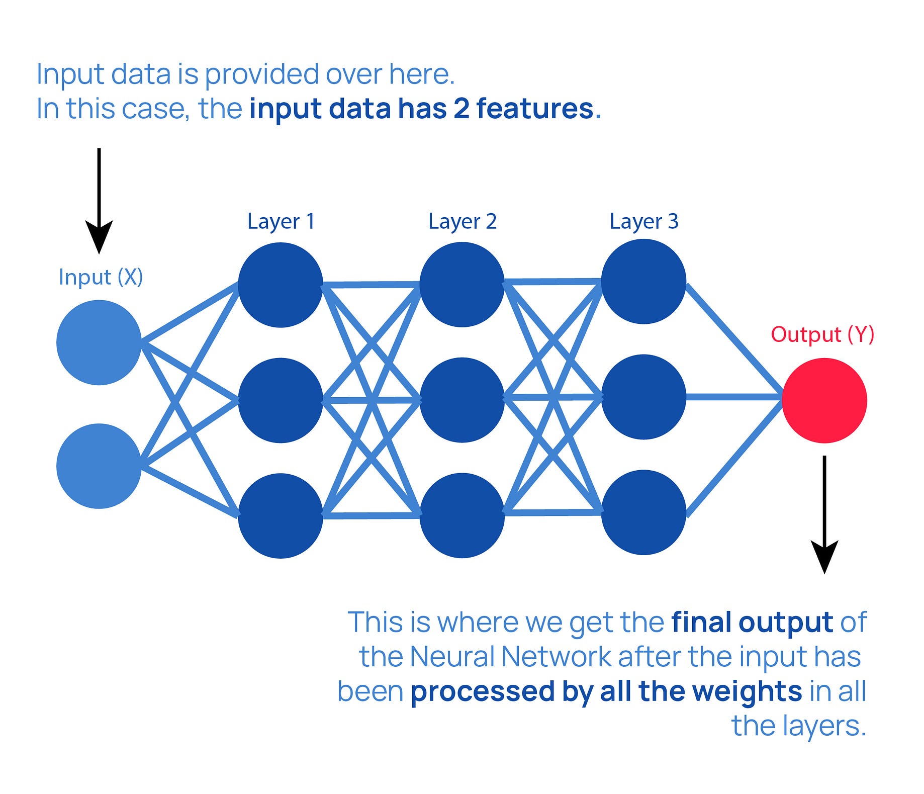
In sequential models, layers are built on top of each other one after the other as shown in the image below.

Functional models are more flexible since they do not attach layers in sequential order.
Here, we will build a sequential model.
Initializing the sequential model
We initialize the sequential model as shown below:
model = keras.Sequential([
    keras.layers.Dense(60, input_dim=60, activation='relu'),
    keras.layers.Dense(30, activation='relu'),
    keras.layers.Dense(15, activation='relu'),
    keras.layers.Dense(1, activation='sigmoid')
])
From the code above, our model will have four layers. These layers are as follows.
Layer 1
The first layer is the input layer for our neural network. It has 60 neurons. We also add activation=relu. We use relu since our output lies between 0 and infinity.
For more information about relu activation function, click here.
Layer 2
This is the first hidden layer containing 30 neurons. We also add activation=relu.
Layer 3
This is the second hidden layer containing 15 neurons. It also uses relu as the activation function.
Layer 4
The 4th layer is the output layer. It has only 1 neuron which is used to produce the prediction results of the model. The layer uses sigmoid as the activation function.
sigmoid activation function is used when the output values that between 0 and 1.
For more information about sigmoid activation function, click here.
The next step is to compile our model.
Model compiling
To compile our model, we have to set the optimizer, the loss, and the metrics for our model to use.
Optimizer
This is used to improve the model performance during training by reducing errors present in the model. We use the adam optimizer.
Metrics
It will be used to determine the model performance so that we know how well the model has learned. We use accuracy to calculate the accuracy score of the model after training.
Loss
It calculates the model error during training. We use binary_crossentropy as our loss because our output is in binary form. The output can either be a 0 or 1.
We add all these using the following code:
model.compile(loss='binary_crossentropy', optimizer='adam', metrics=['accuracy'])
After compiling this model, the next step is to fit the model into our dataset.
Model fitting
During this stage, the model will learn from the training dataset.
model.fit(X_train, y_train, epochs=100, batch_size=8)
We set the number of epochs as 100. The model will iterate through the training dataset 100 times and output the accuracy score after each iteration. This process is shown in the image below:

From the image above, the training score after 100 iterations is 1.00, this represents 100%.
To know if our model is overfitted, let's use the testing dataset to calculate the accuracy score.
Accuracy score using the testing dataset
To check the accuracy score using the testing dataset, use the following code:
model.evaluate(X_test, y_test)
The accuracy score is shown below:

From the image above, the testing score is 0.7692, which represents 76.92%. This shows training accuracy is greater than testing accuracy. The accuracy has drastically dropped from 100% to 76.92%.
Our model performed very well using the training dataset but very poorly using the testing dataset. Therefore, our model is overfitted. We now need to implement dropout regularization to handle this overfitting.
Model with dropout regularization
In dropout regularization, we will add dropout layers in our model. The layers will randomly ignore a certain number of neurons in a neural network during model training.
Let's implement the dropout layers using the following code:
modeld = keras.Sequential([
    keras.layers.Dense(60, input_dim=60, activation='relu'),
    keras.layers.Dropout(0.5),
    keras.layers.Dense(30, activation='relu'),
    keras.layers.Dropout(0.5),
    keras.layers.Dense(15, activation='relu'),
    keras.layers.Dropout(0.5),
    keras.layers.Dense(1, activation='sigmoid')
])
NOTE: We name the new model with dropout regularization as
modeld.
From the code above, we have added a Dropout layer after each Dense layer. We have 3 dropout layers.
1st dropout layer
This layer is added after the input layer where we set the number of neurons to be randomly dropped to 0.5. Therefore, half of the neurons will be randomly dropped from the input layer.
The input layer has 60 neurons, half of these neurons will be randomly dropped.
2nd dropout layer
This layer is added after the 1st hidden layer. We set the number of neurons to be randomly dropped to 0.5. This hidden layer has 30 neurons, half of these neurons will be randomly dropped.
3rd dropout layer
This layer is added after the 2nd hidden layer. We set the number of neurons to be randomly dropped to 0.5. This hidden layer has 15 neurons, half of these neurons will be randomly dropped.
After adding the dropout layers, we can now compile and then fit our model into our dataset. This is done using the following code:
modeld.compile(loss='binary_crossentropy', optimizer='adam', metrics=['accuracy'])
modeld.fit(X_train, y_train, epochs=100, batch_size=8)
This will train our model as shown below.

From the image above, the training score after 100 iterations is 0.9167, this represents 91.67%.
To know if this process has handled overfitting, let's use the testing dataset to calculate the accuracy score.
Using the testing dataset
To calculate the accuracy score using the testing dataset, run this code:
modeld.evaluate(X_test, y_test)
The testing score is shown below:

From the image above our testing score is 0.8077, which represents 80.77%. You can see that by using dropout layers the test accuracy increased from 76.92% to 80.77%.
This is a good improvement and shows that this model performs well in both training and testing. Therefore, using dropout regularization we have handled overfitting in deep learning models.
Conclusion
In this tutorial, we have learned about dropout regularization and how it's used to handle overfitting in deep learning models. We started by differentiating between overfitting and underfitting in machine learning.
We then started to build a model without the dropout regularization technique. The model performed very well using the training dataset but very poorly using the testing dataset.
Finally, we implemented the dropout layers. Using these layers we improved the test accuracy which increased from 76.92% to 80.77%. Therefore, we successfully handled the overfitting.
To get this trained model, click here.
References
- Python code for this tutorial
- Overfitting vs Underfitting
- Techniques used to handle overfitting
- Common activation functions
- TensorFlow documentation
- Keras documentation
Peer Review Contributions by: Srishilesh P S


Cloudzilla is FREE for React and Node.js projects


