Machine Learning

Building A Multiclass Image Classifier Using MobilenetV2 and TensorFlow

In this tutorial, we will build an image-based plant disease classification model using MobileNet-V2 and TensorFlow. We will pre-process the image, segment the objects, extract the features, and finally classify them.  Image classification categorizes the input images into pre-defined labels or categories. The classification models learn from the images dataset that we train, which eventually helps us make predictions.

We have binary and multi-label classifications. Binary classification deals with only two classes/labels, and multi-class classification deals with more than two labels.

In this tutorial, we will focus on multi-class classification. An example would be to classify images of birds into pre-defined birds classes like ostrich, flamingo, hawk, chicken, and owl.

Prerequisites
MobilenetV1 vs MobileNetV2
Why use MobileNetV2?
Implementation
Conclusion
References

Prerequisites

To follow along with this tutorial, the reader should:

Understand the convolutional neural network architecture and how it works.
Know how to build a neural network.
Understand deep learning.
Know how to build a simple image classification model.
Train the deep neural network using Google Colab.

MobilenetV1 vs MobileNetV2

MobileNet uses a Convolutional Neural Network (CNN) architecture model to classify images. It is open-sourced by Google.

Currently, it has two stable versions:

MobilenetV1
MobileNetV2

MobileNet architecture is special because it uses very less computation power to run. This makes it a perfect fit for mobile devices, embedded systems, and computers to run without GPUs.

MobilenetV1 is the first version of the Mobilenet models. It has more complex convolution layers and parameters when compared to MobilenetV2.

MobilenetV2 is the second version of the Mobilenet models. It significantly has a lower number of parameters in the deep neural network. This results in more lightweight deep neural networks. Being lightweight, it is best suited for embedded systems and mobile devices.

MobilenetV2 is a refined version of MobilenetV1. This makes it even more efficient and powerful. The MobileNetV2 models are faster due to the reduced model size and complexity.

MobilenetV2 is a pre-trained model for image classification. Pre-trained models are deep neural networks that are trained using a large images dataset.

Using the pre-trained models, the developers need not build or train the neural network from scratch, thereby saving time for development.

Some of the common pre-trained models for image classification and computer vision are Inceptionv3, ResNet50, VGG-16, EfficientNet, AlexNet, LeNet, and MobileNet.

In this tutorial, we will focus on the second version of Mobilenet as discussed above.

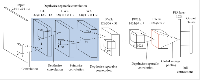
The image below shows the architecture and the number of layers of a pre-trained MobileNetV2 model:

MobileNetV2 convolutional neural network architecture Image source: Medium

To understand CNN's architecture and how it works, read this article.

Number of layers

Number of layers Image source: Medium

Why use MobileNetV2?

It saves time building a neural network from scratch.
MobileNetV2 is trained using a large images dataset. It enables the model to effectively learn, therefore, we can expect accurate results.
It simplifies the process of image processing. Image processing helps transform the image dataset into a format that the model can understand to give more accurate results
MobileNetV2 is lightweight making it have high execution speed.
MobileNetV2 is smaller in size as compared to MobileNetV1, making it more suitable for embedded systems and mobile devices
MobileNetV2 significantly reduces the number of parameters thus making it less complex.
MobilenetV2 can also run on web browsers since the model is lightweight as compared to MobilenetV1. Also, browsers have lower computation power, graphic processing, and storage.

Implementation

Beans images dataset

In this tutorial, we will use the beans images dataset to train the model.

You can find the dataset here.

The dataset contains images of infected and healthy bean leaves. It was collected by taking photos of different infected and healthy bean leaves. Later, the dataset was annotated by experts from the National Crops Resources Research Institute (NaCRRI) in Uganda.

The image below shows a sample of the beans images dataset.

Dataset snip

The multi-class image classification model that we are going to build, will classify each bean leaf into two disease classes/labels or a third class that indicates a healthy leaf.

This model will help farmers to quickly identify infected leaves and reduce significant loss.

We will download the dataset from tensorflow_datasets.

tensorflow_datasets is an open-source repository of datasets used for object detection, object segmentation, image tasks, video tasks, and natural language processing.

Let's import tensorflow_datasets.

import tensorflow_datasets as tfds

We download the beans dataset as follows:

beans_dataset, beans_info = tfds.load(name='beans', with_info=True, as_supervised=True, split=['train','test','validation'])

From the above code snippet:

The load() function will load the beans dataset.
with_info=True will display the beans dataset information and metadata.
as_supervised=True specifies the type of machine learning. We are dealing with supervised machine learning because the beans dataset is labeled.
split will split the dataset into three sets. The sets are for the model to train, test, and validate.

To check the beans dataset, use this code:

beans_info

Beans dataset

The beans dataset contain images of bean leaves taken using mobile phones. It has 3 classes - 2 are beans disease classes and one is healthy bean leaf. The beans disease classes are Angular Leaf Spot and Bean Rust.

The beans dataset has a total of 1295 images. After splitting the dataset, the test set contains 128 samples, the train set contains 1034 samples, and the validation set contains 133 samples.

Showing the beans images

We will visualize some data using the following code:

train, info_train = tfds.load(name='beans', with_info=True, split='test')
tfds.show_examples(info_train,train)

The code will display some of the train images as shown below:

Train images

From this output, Angular Leaf Spot leaves are labeled as 0, Bean Rust as 1, and healthy as 2.

Image preprocessing

Image preprocessing will convert the beans image dataset into a format that the neural network can use. It involves various stages.

Let's create a function that scales the image, normalizes it, and one hot encodes the labels.

def preprocessing(image, label):
  image /= 255.0

  return tf.image.resize(image,[224,224]), tf.one_hot(label, 3)

In the above code, we do the following:

Image normalization converts the output pixel value between 0 and 1.
The preprocessing() function performs normalization by dividing the image pixels by 255.
The function uses tf.image.resize to resize the image to 224,224. It is the image size that MobileNetV2 expects.
The function also one hot encodes the classes using tf.one_hot(label, 3).

One hot encoding is the process of converting categories/classes in a dataset into integer/numeric values which the model understands.

Here, it will convert the classes (Angular Leaf Spot, Bean Rust, healthy), into numerical values (0, 1, 2) respectively.

To understand how one hot encoding works, read this article

Let's now import libraries that we will use for image classification.

Libraries used

Let's import the following:

import tensorflow as tf
import tensorflow_hub as hub
import matplotlib.pylab as plt
import numpy as np

tensorFlow

It is an open-source library used to develop machine learning and deep learning models. It trains deep neural networks with input, hidden, and output layers.

We will use TensorFlow to add custom layers to the pre-trained MobilenetV2. This will help to fine-tune the plant disease classification model and improve its performance.

tensorflow_hub

It is an open-source repository that contains pre-trained models for natural language processing tasks and image classification. We will download the pre-trained MobilenetV2 model from here.

matplotlib.pylab

We will use the library to plot diagrams and visualization of our image dataset. It will show the model prediction results.

numpy

It will convert the image dataset into an array.

Let's now download the pre-trained MobilenetV2 model.

Pre-trained MobilenetV2

We download the pre-trained MobilenetV2 using this code:

mobilenet_v2 = "https://tfhub.dev/google/tf2-preview/mobilenet_v2/feature_vector/4"

As mentioned earlier, the pre-trained MobilenetV2 is created based on the convolutional neural network architecture. This means that MobilenetV2 is made up of many convolution layers, pooling layers, and a fully connected layer.

To use the pre-trained MobilenetV2 layers, use this code:

mobile_net_layers = hub.KerasLayer(mobilenet_v2, input_shape=(224,224,3))

The code above will extract the pre-trained MobilenetV2 layers. It also specifies the size of the beans image that we feed to the pre-trained MobilenetV2.

mobile_net_layers will extract the unique characteristics and features from the beans images. We will then add our custom layers over the pre-trained MobilenetV2 using TensorFlow.

We add the custom layers to fine-tune the existing deep neural network to understand and perform our task (plant disease classification) with better accuracy. The final deep neural network will be made up of the mobile_net_layers and the created custom layers.

To ensure that TensorFlow does not retrain the mobile_net_layers, use this code:

mobile_net_layers.trainable = False

Let's now add our custom layers to the mobile_net_layers.

Adding custom layers using TensorFlow

We will use TensorFlow to build the neural network and add our custom layers. It is done using the following code:

neural_net = tf.keras.Sequential([
  mobile_net_layers,
  tf.keras.layers.Dropout(0.3),
  tf.keras.layers.Dense(3,activation='softmax')
])

We create a Keras Sequential model. The sequential model allows us to build the deep neural network layer-by-layer, by stacking multiple hidden layers on top of each other.

From the above code, we have added the following layers to the deep neural network.

mobile_net_layers contains the pre-trained MobilenetV2 layers.
The dropout layer will handle model overfitting. It ensures the model performs well using both the train and the test images. 0.3% of the neurons will be dropped randomly in training to handle overfitting.
The dense layer is the output layer. It has 3 neurons because the dataset has three predefined classes.
We have also set softmax as the activation function because the dataset has three pre-defined classes.

The softmax activation function is used for multi-label classification, while the sigmoid activation function is used for binary classification.

Let's check the deep neural network architecture.

Deep neural network architecture

We check the model architecture using this code:

neural_net.summary()

Model architecture

From the above image, the model is Keras's sequential model. It also shows all the added layers mobile_net_layers, Dropout, and Dense. The output also shows the following:

Total params: 2,261,827 - These are all the parameters in the deep neural network.
Trainable params: 3,843 - It shows the parameters that the deep neural network will train.
Non-trainable params: 2,257,984 - These are the parameters that the MobilenetV2 model has already trained.

Let's now compile the deep neural network.

Compiling the deep neural network

We compile the deep neural network using the following code:

neural_net.compile(
  model_optimizer=tf.keras.optimizers.Adam(),
  model_loss=tf.keras.losses.CategoricalCrossentropy(from_logits=True),
  model_metrics=['acc'])

We compile the model using the compile function. It has the following parameters:

model_optimizer - It ensures that the model performs well and reduces errors that model_loss generates in training. We set the model_optimizer to Adam.
model_loss - It keeps track of the errors in the model while training. We set the model_loss to CategoricalCrossentropy because the beans dataset has three pre-defined classes.
model_metrics - It checks the deep neural network's performance and calculates the accuracy score. acc will get the accuracy score using the train and the test set.

Let's fit the deep neural network to the train and validation images.

Fitting the deep neural network

The train set will train the deep neural network so that it can learn and understand plant disease classification.

The validation set will adjust and fine-tune the deep neural network parameters. This will produce an improved model with accurate results.

model_fit = neural_net.fit(train, epochs=6, validation_data=validation)

The deep neural network will run for 6 epochs.

Deep neural network training

From the training process above, the first accuracy score is 0.6141 (61.41%). The last accuracy score after the 6 epochs is 0.8878 (88.78%). This shows the accuracy score increases with time.

The validation accuracy score also increases from 0.7368 (73.68%) to 0.8797 (87.97%). Moreover, the model loss reduces from 0.9329 (93.29%) to 0.6898 (68.98). We can see the performance of the model increased with time.

Let's get the test score using the test images.

Test score

To test the model, we use the following code:

test_score=model.evaluate(test)

Test results

The test score is 0.8750 (87.50%). It produces a good score using both the train and test images.

Let's use the trained deep neural network to make predictions.

Using the trained deep neural network to make predictions

It will classify some of the test images into three classes. We select any 10 test images using the following for loop:

for test_sample in beans_dataset[1].take(10):  
  image, label = test_sample[0], test_sample[1]

Let's convert the images into an array.

img = tf.keras.preprocessing.image.img_to_array(image)

It will make the predictions and classify the test images into three classes.

make_predictions = model.predict(image)

Let's use the imported Matplotlib library to visualize the results of the prediction.

print(make_predictions)
plt.figure()
plt.imshow(image)
plt.show()
print(": %s" % info.features["label"].names[label.numpy()])
print(": %s" % info.features["label"].names[np.argmax(make_predictions)])

The code snippet above prints the predicted label and the actual label side by side.

The actual label is the expected bean image class, and the predicted label is the predicted result.

Printed output

From this output, the actual label and the predicted label for both predictions are the same. This shows the deep neural network has made accurate predictions.

Another Output

In this output, the deep neural network has also made accurate predictions.

Conclusion

We have learned how to build a multi-class image classification model using MobileNetV2 and the TensorFlow library. The tutorial also explains the pre-trained MobileNetV2 architecture and how to work with it.

After downloading the pre-trained MobileNetV2, we preprocessed the images and added custom layers using TensorFlow. Using the cleaned images dataset, we trained the deep neural network that classifies images into three classes.

You can check out the full source code here.