Using a Hard Margin vs Soft Margin in Support Vector Machines

Support Vectors are the data points or vectors nearest to the hyperplane and can affect its location. Support vector machines deal with classification and regression problems. <!--more--> They're known as support vectors since they help to stabilize the hyperplane.
The time required to evaluate a big dataset using this technique makes it unfeasible even for smaller datasets.
Table of contents
- Overview on support vector machines
- The role of hard and soft margin in support vector machines
- Support vector machines with a hard margin
- Support vector machines with a soft margin
- Hard margin and soft margin comparisons
Overview on support vector machines
It is possible to utilize vector machines for both classification and regression. Vector Machines are a powerful machine learning method.
Since it has such a significant impact, we must carefully consider the margin that we use to solve a problem.
This section will discuss the distinctions between a hard margin and a soft margin.
Below are the benefits of using support vector machines:
- SVM works effectively whenever we have a clear distinction between classes.
- SVM outperforms other techniques in high-dimensional spaces.
- It's effective when the number of parameters exceeds the sample size.
The role of hard and soft margin in support vector machines
First, consider a set of data that we want to categorize. Based on this knowledge, they may be differentiable, or the splitting of hyperplanes may be non-linear.
We utilize SVMs with a large margin to prevent misclassifications for linear objects.
Soft margins are utilized when a linear border is not usable. They are also applied when we desire to tolerate some errors to increase the generality of the classification system.
Support vector machines with a hard margin
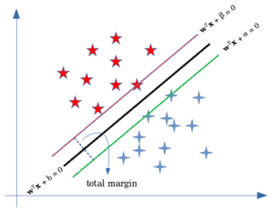
If the hyperplane separating our two classes is defined as wTx + b = 0, then we can define the margin by using two parallel hyperplanes such as wTx + alpha = 0.

SVMs are represented by the green and purple lines in the above picture.
Our goal is to narrow the distance between these two hyperplanes to the greatest extent that is feasible while preventing misclassifications in the hard margin.
We may apply the formula for calculating a point's distance from a plane. In other words, the distances from the blue and red dots, including the ranges between them are shown below:

We must utilize our available area to realize this potential. We can look at alpha = b + 1 and beta = b - 1 without sacrificing generality.
We need to solve the problem in terms of maximization or minimization. To compute gradients, we will use the term in its squared form:

Explanation: The above equation is used to minimize the margin without the loss of generality.
This optimization has several drawbacks. Suppose our classes are -1 and +1 for argument's sake. wx+b>=1, while wx=b=-1 classifies the data as positive.
These two requirements may be linked to a single class. As a solution, our optimization issue would be, as shown below:

Explanation: The above equation is used to express and combine two constraints for optimizing the problem.
This kind of optimization is a primal problem since it always results in the production of a globally minimal value.
We may solve the dual issue by using alpha i Lagrange multipliers in the equation.

Explanation: The above equation solves the problem by introducing Lagrange multipliers and converting it to the dual problem.
The Lagrangian function is the name used to describe this kind of function, which is distinct in terms of (omega) and b which is generated from the SVM's Lagrangian function.

Explanation: When we substitute the above equation in the second term of the Lagrangian function, we would get the dual problem of the SVM.
We will have the SVM dual-issue if we substitute them into the second term of the Lagrangian function.

Therefore, the dual issue is simpler to solve. It can be utilized for non-linear boundaries since it does not require the training data to be divided into dual issues and inner products.
Support vector machines with a soft margin
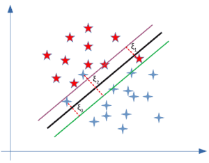
The soft margin SVM optimization method has undergone a few minor tweaks to make it more effective.
The hinge loss function is a type of soft margin loss method.
The hinge loss is a loss function used for classifier training, most notably in support vector machines (SVM) training.
Hinges lose a lot of energy when they are close to the border. If we are on the wrong side of that line, then our instance will be classified wrongly.

Slack variables, or misclassified features, are lost when using hard margin SVM. An example of a major issue in a soft margin is illustrated below:

Explanation: The above equation controls the trade-off between maximizing the margin and minimizing the loss.
We may use the regularization parameter C to control the trade-off between margin expansion and loss reduction.
As shown in the image, several factors have been added to both the fundamental and hard margin problems.
The model is more lenient when misclassifications occur because it contains slack variables. This is illustrated below:

Finally, we may make the following comparison between the two issues in the diagram below:

Explanation: The change in the dual form is merely the upper constraint given to the Lagrange multipliers. This is the only different thing.
Hard margin and soft margin comparisons
Hard margin
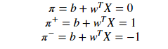
Assume there are three hyperplanes denoted by the letters (π, π+, π-), so that on the positive side of each of them, π+ is parallel to the support vectors, and on the negative side of each of them, π- is parallel to the support vectors.
On the other hand, π is parallel to the support vectors on both of its positive sides.

Image Source: Towards data science
Each hyperplane's equations may well be summarized as follows: (for the sake of point X1)

Image Source: Towards data science
Explanation: As shown above, the equation determines that the product of the actual output and the hyperplane equation is 1, meaning that the point is correctly classified in the positive domain.
For the point X3 is shown below:

Image Source: Towards data science
Explanation: X3 is beyond the hyperplane's domain when it is further away from it. This indicates that the point is positive.
As stated above, if Yi(WT*Xi +b) > 1, then Xi is properly categorized; otherwise, Xi is wrongly classified.
If we add an outlier, our hyperplane becomes worthless since it cannot differentiate linearly separable points. As a result, we must use hard margin SVMs to classify each piece of data.
Soft margin
We presume data can be split linearly, although this might not be the case. This technique eliminates outliers, enabling us to categorize locations almost linearly.
Therefore, the slack variable Xi is generated. If we add ξ to our previous equation, we get:

Image Source: Towards data science
Explanation: The equation above updates the function to skip a few outliers and be able to classify almost linearly separable points.
If ξi= 0, then the points are properly classified. If that's not the case, we receiveξi> 0, which is miscategorized.
If ξi> 0, then the variables will be in the wrong dimension (variable). How to compute the standard deviation error is shown below:

Image Source: Towards data science
Explanation: The above equation calculates the average error of the variable in the incorrect dimension associated with the variable Xi.
As a result, we can express our goal mathematically as:

Image Source: Towards data science
As long as all points are correctly classified, we can find the vector w and b whereby the hyperplane given by w and b maximizes the margin length while minimizing the loss term.
The soft margin method is the name given to this kind of formulation. Hard margins are more exact than soft margins in SVMs because the data is more separable.
When our dataset is split linearly, we strive for a small error margin. Overfitting or excessive sensitivity to outliers is possible because the error margin is so small in certain instances.
We may also employ a softer margin SVM with a larger margin to improve the model's generalization.
Conclusion
In this tutorial, we have looked at the concept of a hard margin and a soft margin SVM and how to use each one of them.
We also discussed the margins for support vector machines.
Happy Learning!
Peer Review Contributions by: Willies Ogola

