Univariate Time Series using Recurrent Neural Networks

A time series consists of various data points sequentially organized in equal intervals over time. A model will analyze the complex patterns and relationships in the time series and predict future values. <!--more--> A time series model can perform various tasks: weather forecasting, stock price prediction, and cryptocurrency prediction. For example, a time series model will analyze the past Bitcoin prices and predict future prices. It helps investors know when to buy and sell Bitcoin to gain profits.

A univariate time series has only a single variable that trains the model. For example, a weather forecast model uses past recorded temperature values to predict future temperatures. We will build a univariate time series model that predicts monthly milk production. We will implement the model using a Recurrent Neural Network (RNN).

There are various types of RNN. We will focus on Long Short-Term Memory (LSTM), which is best suited for time series modeling.

Prerequisites #

• A reader should have the basic knowledge and understanding of the following before implementing the time series model:
• Time series terms and concepts
• A brief introduction to neural networks architecture and concepts
• Know how to build an artificial neural network with Keras
• How to run a Python project in Google Colab

Table of contents #

• Getting started with Recurrent Neural Network (RNN)
• Monthly milk production dataset
• Importing Matplotlib
• Decomposing the time series into components
• Splitting the time series dataset into training and testing dates
• Scaling the time series dataset
• Format the scaled data points into batches
• Building the time series model
• Compiling the sequential time series model
• Fitting the sequential model to the generated batches
• Using the trained sequential model to make predictions
• Plotting the line graph
• Conclusion
• References

Getting started with Recurrent Neural Network (RNN) #

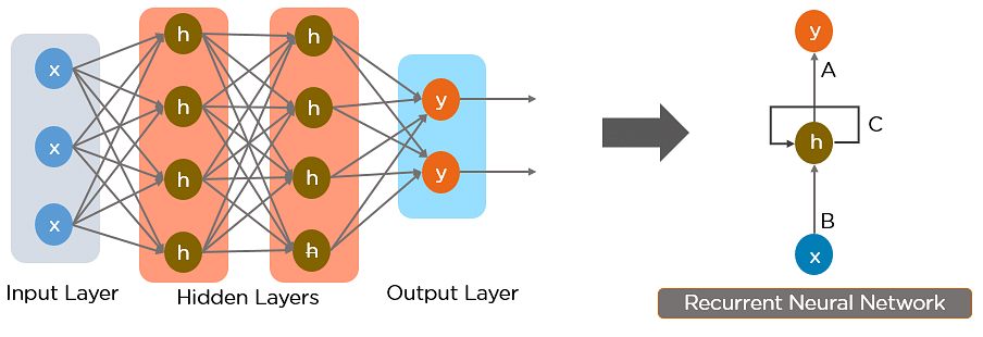
A Recurrent Neural Network is a variant of the typical artificial neural network that can model sequential data. Sequential data depends on historical/past data points to make future predictions.

RNNs use an internal memory that helps them to store information retrieved from the previous data points and use the information to generate other data points. Recurrent neural networks implement a feedback loop within the hidden layers that distinguish them from the traditional artificial neural networks.

The image below shows the distinction between a traditional artificial neural network and a recurrent neural network:

Image Source: Simplilearn

The feedback loops in the hidden layers help the recurrent neural network process and analyze the sequential data for model prediction. The feedback loops also introduce a sequential memory that helps determine the order in which the data values were input into the recurrent neural network. Even though the recurrent neural network is a better improvement than the traditional artificial neural network, it suffers from a long-term dependency problem.

A long-term dependency problem occurs when the sequential memory of the recurrent neural network fails, and the RNN does not determine the order of the data points. The sequential memory fails when the recurrent neural network uses sequential data recorded over a long time, for example, a time series recorded for many years.

The RNN will not remember the information for a long time and therefore lose track of the order of the inputs and how the data points depend on each other. It can not process and analyze the dataset that has longer-term dependencies.

The solution to this problem is to introduce the Long Short-Term Memory (LSTM). The image below shows the basic structure of an LSTM.

Image Source: Medium

LSTM implements a concept known as gates which solves the long-term dependency problem. It, therefore, solves complex deep learning problems that are memory intensive such as speech recognition, time series analysis, machine translation, and other complex natural language processing without losing its internal memory.

To understand the LSTM structure in detail, read this article. In this tutorial, we will implement LSTM for time series modeling. LSTM is much faster and uses less computational power. We will use it to handle the complex patterns in the time series.

Monthly milk production dataset #

We will use the monthly milk production dataset to build the time series model. The dataset is univariate since it only has one variable that trains the time series model. You can download the monthly milk production dataset here

We will load the monthly milk production dataset using Pandas. Let's import this necessary library.

import pandas as pd

To load the monthly milk production dataset, input this code:

df = pd.read_csv('monthly-milk-production-dataset.csv',index_col='Date',parse_dates=True)

We use the parse_dates parameter to enable the Pandas library to recognize the DateTime in the Date column. We can therefore perform time series analysis and operations.

We then convert the dataset to have monthly intervals as follows:

df.index.freq='MS'

To print some of the data points in the monthly milk production dataset, apply this code:

df.head()

It prints the following data points:

The image shows the Date column and its corresponding monthly production. We then plot the monthly milk production dataset using Matplotlib.

Importing Matplotlib #

To import the Matplotlib library, apply this command:

import matplotlib.pyplot as plt

We can then plot the monthly milk production dataset, by applying this code:

df.plot(figsize=(12,6))

It displays the following plot:

From the plot above, we can observe the monthly milk production dataset has seasonality or repeating patterns. It also has a general trend that increases with time.

Decomposing the time series into components #

A time series has various components that make up the general time series pattern. We use seasonal_decompose for time series decomposition.

from statsmodels.tsa.seasonal import seasonal_decompose

To decompose the time series into components, apply this code:

decomposable_components = seasonal_decompose(df['Production'])
decomposable_components.plot()

The code plots the following components:

The code produces the Observed, Trend, Seasonal, and Residual components:

• Observed: It shows the general pattern of the monthly milk production dataset.
• Trend: It shows the time series uptrend over time.
• Seasonal: It shows the seasonality or the repeating patterns in the time series.
• Residual: It shows the time series after removing the seasonality and trend components.

Splitting the time series dataset into training and testing dates #

We have to split the time series dataset into training and testing dates. We will use the training dates and their corresponding monthly production for model training. We will then use testing dates for model prediction.

train_dates = df.iloc[:156]
test_dates = df.iloc[156:]

We will use the first 156 months to be the training dates. The remaining months will be the testing dates.

Scaling the time series dataset #

We have to convert the time series dataset into a scale between 0 and 1. It will ensure that all the data points fit into the LSTM. We will use MinMaxScaler for scaling:

from sklearn.preprocessing import MinMaxScaler

To initialize the scaling method, execute this code:

scaler = MinMaxScaler()

We fit our scaler to both the training and testing dates:

scaler.fit(train_dates)
scaler.fit(test_dates)

We then call the transform method to convert the training and testing dates:

scaled_train_dates = scaler.transform(train_dates)
scaled_test_dates = scaler.transform(test_dates)

To see some of the scaled time series values, execute this code:

scaled_train_dates[:10]

The code displays the following scaled points:

The output shows the scaled data points that lie between 0 and 1.

Format the scaled data points into batches #

We have to take the scaled data points and break them into batches. The batches are a sequence of values that the LSTM will use as inputs during the training phase. We use the TimeseriesGenerator class to generate the dataset batches.

We can import this necessary library as follows:

from keras.preprocessing.sequence import TimeseriesGenerator

We define the size of each batch as follows:

n_input = 12
n_features = 1

Each batch will have 12 scaled data points (n_input = 12). We then set the number of variables in the time series dataset using n_features. We set the value to one since we are dealing with a univariate time series.

Let's apply TimeseriesGenerator to our scaled data points:

generated_batches = TimeseriesGenerator(scaled_train_dates, scaled_test_dates, length=n_input, batch_size=1)

The code will apply the class function to both the training and testing dates. Each batch will have a specific size.

Building the time series model #

We will build a sequential time series model using LSTM. A sequential model will enable us to add multiple layers one after the other (layer by layer). The LSTM will be the input layer of the sequential model.

We will import the LSTM from Keras and add it directly as the input layer of the sequential model. We will then add the output layer of the sequential model using the Dense layer. Let's import the LSTM, Sequential model, and the Dense layer from Keras.

from keras.layers import LSTM
from keras.models import Sequential
from keras.layers import Dense

Let's initialize the Sequential model as follows:

lstm_model = Sequential()

After this, we add the LSTM layer as follows:

lstm_model.add(LSTM(100, activation='relu', input_shape=(n_input, n_features)))

The LSTM layer will have 100 neurons. It uses relu as an activation function because the output of this layer will be between 0 and infinite positive time series values. It uses the generated dataset batches as inputs. The model will then use the Dense layer to output the predicted time series values.

Let's add the Dense layer as follows:

lstm_model.add(Dense(1))

The Dense layer will have only one neuron to output the predicted monthly milk production.

Compiling the sequential time series model #

To compile the sequential time series model, apply this code:

lstm_model.compile(optimizer='adam', loss='mse')

We compile the sequential time series model using the compile function. For the compilation process to work, we have passed the following parameters.

• optimizer: It will improve and enhance the performance of the sequential time series model. We pass adam as the optimizer for the model compilation process to work.

• loss: It will keep track and calculate all the model errors. We pass mse as the parameter value.

Printing the summary of the sequential time series model #

To print the sequential time series model summary, apply this code:

lstm_model.summary()

The code displays the following:

The summary shows the layers in the compiled sequential time series model and the parameters. Let's fit the sequential model to the generated batches.

Fitting the sequential model to the generated batches #

To fit the sequential model, apply this code:

lstm_model.fit(generated_batches,epochs=100)

The generated batches will train and test the sequential model. We apply 100 epochs to reduce the errors (loss) of the sequential model. The sequential model will run 100 times through the generated batches.

The code above will give the following output:

We have trained the sequential model using the generated batches. From the output, the model loss has reduced with time. Let's use the trained sequential model to make predictions.

Using the trained sequential model to make predictions #

The trained sequential model will use the testing dates to predict the monthly milk production. We have to reshape the scaled test time series values to have the original format.

prediction_result = []

test_batches = scaled_train_dates[-n_input:]
reshaping_batches = test_batches.reshape((1, n_input, n_features))

The reshape method will reshape the testing time series values. We will then save the predicted output in the prediction_result variable. We then use the following for loop function to loop through the testing dataset. It will analyze the data points and make predictions.

for i in range(len(test_dates)):

    predicted_output = lstm_model.predict(reshaping_batches )[0]

    prediction_result.append(predicted_output) 

    reshaping_batches = np.append(reshaping_batches [:,1:,:],[[predicted_output]],axis=1)

The check the predicted results, apply this code:

prediction_result

The code displays the following predicted values:

The final step is to use Matplotlib to plot a line graph to show the actual data points in the testing dataset and the predicted data points. The line graph will evaluate the performance of the sequential time series model.

Plotting the line graph #

To plot the line graph, execute this code snippet:

actual_values = scaler.inverse_transform(prediction_result)
test_dates['Predictions'] = actual_values
test_dates.plot(figsize=(14,5))

The code snippet above plots the following line graph:

The line graph shows the actual monthly milk production and the predicted monthly milk production.

• The orange line shows the predicted milk production.
• The blue line shows the actual milk production.

If we observe the two lines, they maintain the same pattern. Also, these lines are close two each other. It implies the sequential time series model was well trained and can make accurate predictions (the predicted values lie within the actual values).

Conclusion #

In this tutorial, we have built a univariate time series that predicts monthly milk production. We implemented the model using LSTM since it is best suited for time series modeling.

We explained the difference between RNN and LSTM and how the LSTM solves the long-term dependency problem. We imported LSTM from Keras and used it to build the sequential time series model. We finally used the line graph to evaluate the performance of the sequential time series model.

Please check out the complete Python Code for the univariate time series model here.

Happy coding!

References #

• TimeSeriesGenerator
• Keras API
• Python LSTM
• Recurrent Neural Network architecture
• Types of RNN

---

Peer Review Contributions by: Willies Ogola