Perceptron Algorithm - A Hands On Introduction

Perceptrons were one of the first algorithms discovered in the field of AI. Its big significance was that it raised the hopes and expectations for the field of neural networks. Inspired by the neurons in the brain, the attempt to create a perceptron succeeded in modeling linear decision boundaries. <!--more--> A linear decision boundary can be visualized as a straight line demarcating the two classes. In this article, we will understand the theory behind the perceptrons and code a perceptron from scratch.

We will also look at the perceptron's limitations and how it was overcome in the years that followed.

Goals #

This article will explain what perceptrons are, and we will implement the perceptron model from scratch using Numpy. For a quick refresher on Numpy, refer to this article.

By the end of the article, you'll be able to code a perceptron, appreciate the significance of the model and, understand how it helped transform the field of neural networks as we know it.

Perceptron #

Frank Rosenblatt developed the perceptron in the mid-1950s, which was based on the McCulloch-Pitts model. The McCulloch-Pitts model was proposed by the legendary-duo Warren Sturgis McCulloch and Walter Pitts. Although these models are no longer in use today, they paved the way for research for many years to come.

The perceptron is a mathematical model that accepts multiple inputs and outputs a single value. Inside the perceptron, various mathematical operations are used to understand the data being fed to it.

Structure #

Let's consider the structure of the perceptron. The perceptron has four key components to it:

1. Inputs
2. Weights
3. Weighted Sum
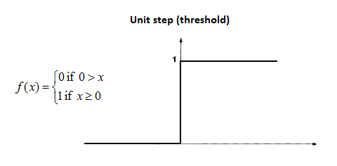
4. Thresholding using the unit-step function

Image Source

The inputs $x1, x2, x3$, represent the features of the data. For example, given a classifying task based on gender, the inputs can be features such as long/short hair, type of dress, facial features, etc. The input features are numbers in the range $(-\infin,\infin)$.

The inputs were sent through a weighted sum function. This was the first time weights were introduced. The McCullock-Pitts model only used the features to compute the confidence scores.

Using the weighted summing technique, the perceptron had a learnable parameter. By adjusting the weights, the perceptron could differentiate between two classes and thus model the classes. The idea of using weights to parameterize a machine learning model originated here.

The weighted sum is sent through the thresholding function. The output of the thresholding functions is the output of the perceptron. The output indicates the confidence of the prediction. The larger the numerical value of the output, the greater the confidence of the prediction.

Image Source

Update Rule #

How do humans learn? We make a mistake, correct ourselves, and, if lucky, make more mistakes. Similarly, the majority of the learning algorithms learn through iterative steps. Iterative steps refer to the gradual learning by the algorithm upon seeing new data samples.

We will consider the batch update rule. That is, the algorithm computes the difference between the predicted value and the actual value. The difference is defined as an error. If the predicted value is the same as the real value, then the error is 0; otherwise, it's a non-zero number. Once the errors have been computed for all the data samples, then the parameters are updated. The parameters define the learning model, and in this case, it's the weights.

The learning update rule is given as follows:

$weights_j:= weights_j + \alpha(y^{(i)}-h_\theta(x^{(i)})x_j^{(i)}$

The updated weights are changed by the difference in the actual output value, denoted by $y^{(i)}$, and the predicted output, represented by $h_\theta(x^{(i)})$.

The need to update the weights #

The weights need to be updated so that error in the prediction decreases. The update rule is computing the error and changing the weights based on the error's sign and magnitude. The learning rate denoted by $\alpha$ decides the scale of impact of the error.

If the learning rate is high, small errors can cause considerable shifts in the values of weights. On the contrary, if the learning rate is small, significant errors cause minimal changes in the weights. Therefore, it's necessary to find the right balance between the two extremes. For more information related to learning rates, refer to this article.

Code #

We have just gone through the code of the first-ever model to learn patterns in data. We must code the same to get a better understanding of the concepts we just went through.

Let's define a class called PerceptronClass and its methods:

1. __init__: Let's define the __init__ method and initialize the following parameters:

   • weights: The weights are the parameters that the model learns.
   • bias: Bias is the intercept that helps the learned decision boundary translate across the axes.
   • learning_rate: As mentioned earlier, the learning rate is used to control the error's impact on the updated weights. We set it to 0.001 for all practical purposes.
   • num_iterations: The number of iterations the algorithm is trained for. Each time the algorithm sees a data sample, it's regarded as one iteration.

2. unit_step_function: The threshold function blocks all values less than 0 and allows all values greater than 0. Therefore, any negative value is multiplied by 0 to stop it from passing through.

3. fit: The fit method goes through the following set of steps."

   • Initialize parameters randomly: Weights and Bias.
   • Predict the output and pass it through the threshold function.
   • Apply the update rule, and update the weights and the bias.

4. predict: The predict method is used to return the model's output on unseen data. Using this method, we compute the accuracy of the perceptron model.

import numpy as np

class PerceptronClass:

    def __init__(self, learning_rate=0.01, num_iters=1000):
        self.weights = None
        self.bias = None
        self.num_iterations = num_iters
        self.lr = learning_rate

    def _unit_step_func(self, x):
        return np.where(x >= 0, 1, 0)

    def fit(self, X, y):
        n_samples, n_features = X.shape

        # init parameters
        self.weights = np.zeros(n_features)
        self.bias = 0

        y_ = np.array([1 if i > 0 else 0 for i in y])

        for _ in range(self.num_iterations):

            for idx, x_i in enumerate(X):

                linear_output = np.dot(x_i, self.weights) + self.bias
                y_predicted = self._unit_step_func(linear_output)

                # Perceptron weight update rule:
                # weight := weight - learning_rate*(error)
                update = self.lr * (y_predicted - y_[idx])

                self.weights -= update * x_i
                self.bias -= update

    def predict(self, X):
        linear_output = np.dot(X, self.weights) + self.bias
        y_predicted = self._unit_step_func(linear_output)
        return y_predicted

from sklearn.datasets import load_iris
from sklearn.model_selection import train_test_split
from sklearn.metrics import accuracy_score

data = load_iris()
X, y = data.data, data.target
X_train, X_test, Y_train, Y_test = train_test_split(X,y, test_size=0.2)

perceptron = PerceptronClass()
perceptron.fit(X_train,Y_train)

y_predicted = perceptron.predict(X_test)
y_predicted_train = perceptron.predict(X_train)

acc = accuracy_score(y_predicted,Y_test)
train_acc = accuracy_score(y_predicted_train,Y_train)

print("Training Accuracy: ", train_acc)
print("Testing Accuracy: ", acc)

We are using the Iris dataset available in sklearn.datasets module. We fit the model to the training data and test it on test data using the predict method. The output of the predict method, named y_predicted is compared with the actual outputs to obtain the test accuracy.

We get a test accuracy varying around 67%. The test accuracy is computed on unseen data, whereas the training accuracy is calculated on the data that the algorithm was trained on.

The training accuracy averages around 65%. The test accuracy is greater than the training accuracy. This indicates that the model can (be tweaked to) learn better, given changes are made in the hyper-parameters such as the learning rates and the number of iterations.

It will be a fun challenge to change the values of the learning rate and the number of iterations and observe their effect on the accuracies.

I have attached a screenshot of the terminal capturing the training and test accuracies.

Code Output

Disadvantages #

The perceptron model showed that it could model datasets with linear decision boundaries. Even though it introduced the concept of weights, it had its own set of disadvantages:

1. The algorithm doesn't scale well with massive datasets.
2. It fails to capture non-linear decision boundaries. Most of the data available is non-linear.
3. The step function makes updating the weights inefficient due to the abrupt change in value at 0.

To tackle the problems above, a lot of modifications have been made. The unit-step function has been replaced with a continuous function called the sigmoid function.

The learning algorithms have been updated to consider the error surfaces' derivatives, rather than only the errors. To ensure non-linearity, various activation functions have been implemented as well.

Conclusion #

In this article, we have looked at the perceptron model in great detail. The perceptron model is an inspiring piece of work. I hope you enjoyed reading the article as much as I enjoyed writing it. I would love to know about your experiments with the perceptron model and any feedback. Do connect with me on Linkedin.

<!-- MathJax script --> <script type="text/javascript" async src="https://cdnjs.cloudflare.com/ajax/libs/mathjax/2.7.1/MathJax.js?config=TeX-AMS-MML_HTMLorMML"> MathJax.Hub.Config({ tex2jax: { inlineMath: [['$','$'], ['\(','\)']], displayMath: [['$$','$$']], processEscapes: true, processEnvironments: true, skipTags: ['script', 'noscript', 'style', 'textarea', 'pre'], TeX: { equationNumbers: { autoNumber: "AMS" }, extensions: ["AMSmath.js", "AMSsymbols.js"] } } }); MathJax.Hub.Queue(function() { // Fix <code> tags after MathJax finishes running. This is a // hack to overcome a shortcoming of Markdown. Discussion at // https://github.com/mojombo/jekyll/issues/199 var all = MathJax.Hub.getAllJax(), i; for(i = 0; i < all.length; i += 1) { all[i].SourceElement().parentNode.className += ' has-jax'; } }); MathJax.Hub.Config({ // Autonumbering by mathjax TeX: { equationNumbers: { autoNumber: "AMS" } } }); </script>