Bagging algorithms in Python

We can either use a single algorithm or combine multiple algorithms in building a machine learning model. Using multiple algorithms is known as ensemble learning. <!--more--> Ensemble learning gives better prediction results than single algorithms. The most common types of ensemble learning techniques are bagging and boosting.

In Bagging, multiple homogenous algorithms are trained independently and combined afterward to determine the model's average.

Boosting is an ensemble technique, where we train multiple homogenous algorithms sequentially. These individual algorithms create a final model with the best results. The performance of one algorithm is influenced by the performance of the previously built algorithm.

This tutorial will use the two approaches in building a machine learning model.

In the first approach, we will use a single algorithm known as the Decision Tree Classifier to build and find the accuracy of a model.

In the second approach, we will use the Bagging Classifier and the Random Forest Classifier to build the same model and find its accuracy.

Table of contents #

• Prerequisites
• Bagging vs Boosting
• How Bagging works
• Bootstrapping
• Parallel training
• Aggregation
• Benefits of using Bagging algorithms
• Dataset used
• Loading the dataset
• Dataset scaling
• Splitting the dataset
• Model building using Decision Tree Classifier
• Getting the mean accuracy score
• Implementing the bagging algorithms
• Building the model using Bagging Classifier
• Fitting the model
• Accuracy score
• Building the model using Random Forest Classifier
• Conclusion
• References

Prerequisites #

To follow along with this tutorial, the reader should know the following:

• Python programming.
• Machine learning workflows.
• Machine learning in Python using Scikit-learn.
• Data analysis using Pandas.

NOTE: In this tutorial, we will use Google Colab notebook.

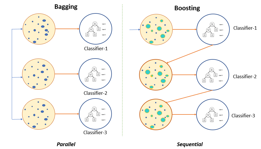
Bagging vs Boosting #

As mentioned above, in Bagging, multiple homogenous algorithms are trained independently in parallel, while in Boosting, multiple homogenous algorithms are trained sequentially. The image below shows the difference between Bagging and Boosting.

Image Source: Pluralsight

In this tutorial, we will only be focusing on implementing Bagging algorithms. To implement Boosting algorithms, read this article.

How Bagging works #

The Bagging technique is also known as Bootstrap Aggregation and can be used to solve both classification and regression problems. In addition, Bagging algorithms improve a model's accuracy score.

These algorithms prevent model overfitting and reduce variance.

Overfitting is when the model performs well using the training dataset but poorly using the testing dataset, meaning the model will not be able to make accurate predictions.

Variance is used to describe the changes within a model. For example, a variance occurs when you train the model using different splits.

Bagging algorithms are used to produce a model with low variance. To understand variance in machine learning, read this article.

Bagging comprises three processes: bootstrapping, parallel training, and aggregation.

Bootstrapping #

Bootstrapping is a data sampling technique used to create samples from the training dataset.

Bootstrapping samples the rows and columns of the training dataset with replacement randomly. We can select the same data samples multiple times using sampling with replacement.

The bootstrapping process generates multiple subsets from the original datasets. The multiple subsets have equal tuples and can be used as a training dataset.

The image below shows the bootstrapping process:

Image Source: Data Aspirant

Parallel training #

The process of bootstrapping generates multiple subsets. On each subset, a machine learning algorithm is fitted.

The fitting algorithm is trained using multiple subsets to produce various models. The various models produced are called weak learners or base models.

We will have multiple base models trained in parallel by this stage.

The image below shows the parallel training process:

Image Source: Data Aspirant

Aggregation #

Aggregation is the last stage in Bagging. The multiple predictions made by the base models are combined to produce a single final model. The final model will have low variance and a high accuracy score.

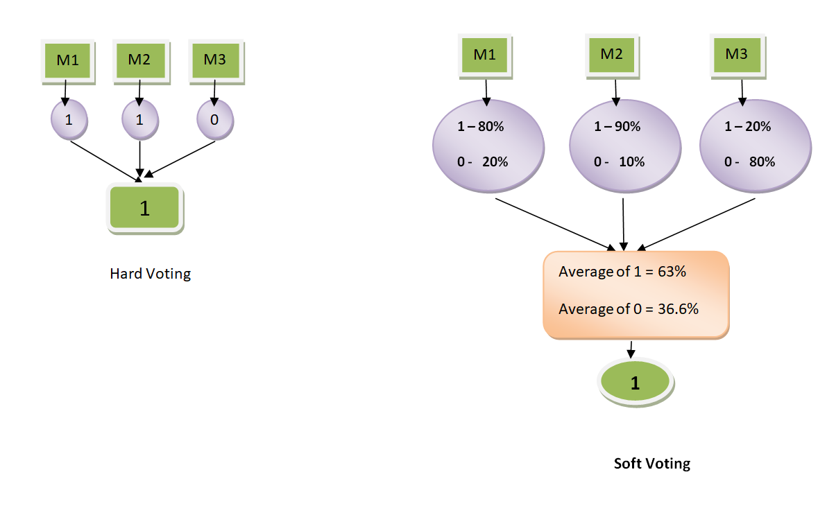
The final model is produced depending on the voting technique used. We have two common voting techniques used, hard voting and soft voting.

Hard Voting

Hard voting is also known as majority voting. Hard voting is majorly used when dealing with a classification problem.

In classification problems, the prediction made by each base model is seen as a vote. This is because the most common prediction made by the base models is the right prediction.

The image below shows the hard voting process:

Image Source: Data Aspirant

Soft Voting

Soft voting is majorly used when dealing with a regression problem. In soft voting, we find the average of the predictions made by the base models. The average value is what is taken as the prediction result.

The image below shows the hard vs soft voting side-by-side:

Image Source: Medium

The image below further shows the process of Bagging. Again, the image clearly describes how each process is done.

Benefits of using Bagging algorithms #

• Bagging algorithms improve the model's accuracy score.
• Bagging algorithms can handle overfitting.
• Bagging algorithms reduce bias and variance errors.
• Bagging can easily be implemented and produce more robust models.

Now that we have discussed the theory, let us implement the Bagging algorithm using Python.

Dataset used #

We will use the diabetes dataset to predict if a person has diabetes or not. The collected dataset has Age and blood pressure features, which help the model determine if the person has diabetes.

To download the diabetes dataset, click here.

Loading the Dataset #

We will use the Pandas library to load the dataset we downloaded using the link above.

Let us import Pandas.

import pandas as pd

To load the dataset, use this code:

df = pd.read_csv("/content/diabetes.csv")

Lets now see how our dataset is structured using the following code:

df.head()

The dataset structure is shown in the image below:

Our dataset has columns such as Age and blood pressure from the image above.

The features will be used as input for the model. The last column labeled Outcome will be an output column. The Outcome column is either labeled 0(non-diabetic) or 1(diabetic).

Let us check for missing values in this dataset.

Checking for missing values #

Missing values makes the dataset incomplete. The dataset with missing values leads to inconsistent results and poor model performance.

To check for missing values, use this code:

df.isnull().sum()

The output is shown below:

From the image above, there are no missing values. Therefore, our dataset is complete and ready for use.

Adding x and y variables #

We need to specify the x and y variables. The x variable will hold all the input columns, while the y variable will hold the output column.

In our case, our output column is the Output column. The remaining columns will be used as model inputs.

We add the x and y variables using the following code:

X = df.drop("Outcome",axis="columns")
y = df.Outcome

The next step is to scale our dataset.

Dataset scaling #

Dataset scaling is transforming a dataset to fit within a specific range. For example, you can scale a dataset to fit within a range of 0-1, -1-1, or 0-100.

Dataset scaling ensures that no data point value is left out during model training.

To understand the concept of dataset scaling better, read this article

We have different scales for dataset scaling. In our case, we use the StandardScaler to scale our dataset.

To further understand how the StandardScaler works to perform scaling, click here.

Let us import the StandardScaler

from sklearn.preprocessing import StandardScaler

To scale our input columns(The x variable), use this code:

scaler = StandardScaler()
X_scaled = scaler.fit_transform(X)

If the code is executed, it will scale the entire dataset. To see some of the scaled datasets, use this code:

X_scaled[:3]

The output will show the 4th row of the scaled dataset:

After scaling the dataset, we can split the scaled dataset.

Splitting the Dataset #

We will split the scaled dataset into training and testing. To split the dataset, we will use the train_test_split method.

from sklearn.model_selection import train_test_split

To perform the splitting, use this code:

X_train, X_test, y_train, y_test = train_test_split(X_scaled, y, stratify=y, random_state=10)

The code above will use the default splitting ratio when splitting the dataset. 80% of the data will be the training set and 20% the testing set.

To check the number of data samples in the training set, use this code:

X_train.shape

The output is shown below:

(576, 8)

We can also see the size of the testing dataset using the following code:

X_test.shape

The output is shown below:

(192, 8)

Model building using Decision Tree Classifier #

The decision tree classifier is the Scikit-learn algorithm used for classification. To import this algorithm, use this code:

from sklearn.tree import DecisionTreeClassifier

We will use k-fold cross-validation to build our decision tree classifier. In addition, K-fold cross-validation allows us to split our dataset into various subsets or portions.

The model is then trained using each subset and gets the accuracy scores after each iteration. Finally, the mean accuracy score is calculated. K refers to the number of subsets/portions we split the dataset.

For a detailed understanding of K-fold cross-validation, read this guide.

Let us import the method that will help to perform K-fold cross-validation.

from sklearn.model_selection import cross_val_score

To use the cross_val_score method, run this code:

scores = cross_val_score(DecisionTreeClassifier(), X, y, cv=5)
scores

In the code above, we will split the dataset into five folds. It produces the model accuracy score after each iteration, as shown in the output below:

array([0.69480519, 0.68181818, 0.71428571, 0.77777778, 0.73856209])

Getting the Mean Accuracy Score #

The mean score is obtained using the following code:

scores.mean()

The output is shown below:

0.7214497920380273

Using the cross-validation score, we get the accuracy score to be 0.7214497920380273. We can build the same model using the bagging algorithms to compare the accuracy scores.

Implementing the Bagging algorithms #

Let us first build the model using the BaggingClassifier.

Building the model using Bagging Classifier #

The BaggingClassifier classifier will follow all the bagging steps and build an optimized model. The BaggingClassifier will fit the weak/base learners on the randomly sampled subsets.

Next, it will use the voting techniques to produce an aggregated final model. Finally, we will use the DecisionTreeClassifier algorithm as our weak/base learners.

To import the BaggingClassifier, use this code:

from sklearn.ensemble import BaggingClassifier

To use this model, use this code:

bag_model = BaggingClassifier(
base_estimator=DecisionTreeClassifier(), 
n_estimators=100, 
max_samples=0.8, 
bootstrap=True,
oob_score=True,
random_state=0
)

In the code snippet above, we have used the following parameters: base_estimator - This represents the algorithm used as the base/weak learners. We will use the DecisionTreeClassifier algorithm as our weak/base learners.

n_estimators - This represents the number of weak learners used. We will use 100 decision trees to build the bagging model.

max_samples - The maximum number of data that is sampled from the training set. We use 80% of the training dataset for resampling.

bootstrap - Allows for resampling of the training dataset without replacement.

oob_score - Used to compute the model's accuracy score after training.

random_state - Allows us to reproduce the same dataset samples. Furthermore, it ensures that the same ratio is used when producing the multiple subsets.

The next step is to fit the initialized model into our training set.

Fitting the Model #

Fitting will enable the model to learn from the training dataset to understand the dataset and gain helpful insight.

To fit the model, use this code:

bag_model.fit(X_train, y_train)

Finally, let us calculate the model accuracy score.

Accuracy Score #

To get the accuracy score, run this code:

bag_model.oob_score_

The accuracy score is shown below:

0.7534722222222222

The model improves the accuracy score. For example, the accuracy score improved from 0.7214497920380273 to 0.7534722222222222.

We can also check the accuracy score using the testing dataset to determine if our model is overfitting. To get the accuracy score, use this code:

bag_model.score(X_test, y_test)

The output is shown below:

0.7760416666666666

The accuracy score shows that our model is not overfitting. Overfitting occurs when we get a lower accuracy when using the testing dataset.

Let us now use the Random Forest Classifier.

Building the model using Random Forest Classifier #

Random Forest Classifier has several decision trees trained on the various subsets. This algorithm is a typical example of a bagging algorithm.

Random Forests uses bagging underneath to sample the dataset with replacement randomly. Random Forests samples not only data rows but also columns. It also follows the bagging steps to produce an aggregated final model.

Let us import the Random Forest Classifier.

from sklearn.ensemble import RandomForestClassifier

To use the RandomForestClassifier algorithm, run this code:

scores = cross_val_score(RandomForestClassifier(n_estimators=50), X, y, cv=5)

We have also used the K-fold cross-validation to train the model. To get the mean accuracy score, use this code snippet:

scores.mean()

The output is shown below:

0.7618029029793736

The accuracy score is high, showing that the bagging algorithms increase the model accuracy score. It also prevents model overfitting.

Conclusion #

This tutorial guided a reader on how to implement bagging algorithms in Python. We discussed the difference between Bagging and boosting. We also went through all the steps involved in Bagging, clearly illustrating how each step works.

Furthermore, we built a diabetes classification model using both a single algorithm and bagging algorithms. The bagging algorithms produced a model with a higher accuracy score, indicating that bagging algorithms are best suited for building better models.

To get the Python code, click here.

References #

• Bootstrap aggregating.
• How bagging works.
• Ensemble Learning: Bagging & Boosting.
• Ensemble methods.
• Cross-validation.
• Boosting Algorithms in Python
• Scikit-learn documentation.

---

Peer Review Contributions by: Jerim Kaura