Hyperparameter Tuning of Machine Learning Model in Python

Hyperparameters are parameters that can be fine-tuned and adjusted. This increases the accuracy score of a machine learning model. Machine algorithms such as Random forest, K-Nearest Neighbor and Decison trees have parameters that can be fine-tuned to achieve an optimized model. <!--more--> This tutorial will increase the model's accuracy score. This ensures that the model makes accurate predictions. We will also create a list of all the possible values for hyperparameters and iterate through the values, finding all the hyperparameters combinations. We then calculate and record the performance of each parameter. Finally, we use hyperparameters that will provide an optimal model.

Table of contents #

• Prerequisites
• Hyperparameter tuning techniques
• Generate synthetic dataset
• Examine the data dimension
• Splitting our dataset
• Building a machine learning model using Random Forest
• Model fitting
• Making predictions using the test dataset
• Accuracy score
• Getting started with hyperparameter tuning
• Creating the grid
• The best parameters for the model
• Conclusion
• References

Prerequisites #

To follow along, a reader is required:

• To have Python installed.
• To know Python programming.
• To know how to train a machine learning model.
• To know how to work with the Scikit-learn library.
• To know how to work with Google Colab notebook.

Hyperparameter tuning techniques #

Choosing the optimal hyperparameters is important in building a successful machine learning model. Hyperparameters have a great impact on the machine learning algorithms used. Manual searching for the best hyper-parameter is a tedious process. Therefore, we need techniques that simplify this work.

These techniques are as follows:

Grid search #

This is a brute force searching technique. In this technique, we create a list of all the combination values for hyperparameters. We then iterate through all hyperparameters. Finally, it records the best performing hyperparameters used in model training. This is shown below:

Image source: Medium

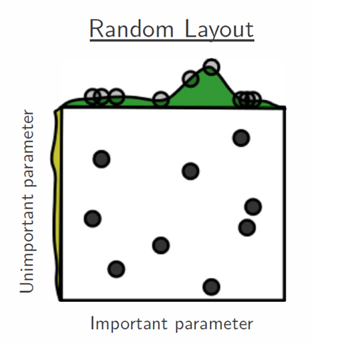
Random search #

We also create a list of all the combination values for hyperparameters in this technique. It's similar to grid search, but it uses random search instead of exhaustive search. For example, instead of checking all the 10,000 possible values of hyperparameters, we can only check 500 random parameters. This is shown below:

Image source: Medium

Bayesian optimization #

This technique uses probability to find a model with the minimum loss function. It does this by mapping the hyperparameters to the function that will produce an optimal model. Bayesian Optimization ensures that the process takes the minimum number of steps.

Gradient-based optimization #

It is best used with the gradient descent algorithm. It fine-tunes the parameters for the gradient descent algorithm to produce an optimal model.

Evolutionary optimization #

This technique uses the concept of natural selection in hyperparameter tuning. It uses the concept of the evolution process and survival of the fittest by Charles Darwin.

In this tutorial, we will implement the first approach of hyperparameter tuning: the Grid Search Technique.

Let's now start with the practical approach.

Generate synthetic dataset #

A synthetic dataset is artificially manufactured. It's used to easily explain certain machine learning concepts, such as hyperparameter tuning.

Let's import make_classification, the machine learning package used to generate the synthetic dataset.

from sklearn.datasets import make_classification

We now need to specify how our generated dataset will be structured.

X, Y = make_classification(n_samples=200, n_classes=2, n_features=10, n_redundant=0, random_state=1)

Let's explain this code as follows:

• n_samples=200: This represents the number of data samples in our dataset, which will be 200.

• n_classes=2: This is the target output. It can either be a 1 or 0. This is the prediction output of the model.

• n_features=10: These are the independent variables that are used as input for the model. The model will have a total of 10 input columns.

• n_redundant=0: This specifies the number of repeated data points in the dataset.

• random_state=1 It is used to set the seeding factor used to generate our dataset randomly. This ensures that the model results can be reproduced and applied elsewhere.

Examine the data dimension #

This is used to check the size and structure of our dataset. To check the data dimension, run this code:

X.shape, Y.shape

The output is shown below:

((200, 10), (200,))

X.shape is used to represent the input variables (200, 10). This shows that our input has 200 data points and 10 input columns.

Y.shape is used to represent the output/target variable (200,). This shows that our output has 200 data points and a 1 output column. The output column will be used to give the prediction results.

Let's split our dataset.

Splitting our dataset #

Let's import the package required for dataset splitting.

from sklearn.model_selection import train_test_split

train_test_split will be used to split our dataset. 80% of the dataset will go to the training subset and 20% to the testing subset. This is done using a test_size=0.2.

X_train, X_test, Y_train, Y_test = train_test_split(X, Y, test_size=0.2)

Let's examine our training subset. To check the size of the training dataset, run this code:

X_train.shape, Y_train.shape

The output below represents 80% of the dataset.

((160, 10), (160,))

Let's examine our testing subset. To check the size of the testing dataset, run this code:

X_test.shape, Y_test.shape

The output below represents 20% of the dataset.

((40, 10), (40,))

We will build a machine learning model using a random forest algorithm. After building the model, we will fine-tune the algorithm's parameters to produce an optimal model.

Let's build our model.

Building a machine learning model using Random Forest #

Let's import the necessary machine learning packages.

from sklearn.ensemble import RandomForestClassifier
from sklearn.metrics import accuracy_score

Let's explore what we have imported:

• RandomForestClassifier: This is the classification algorithm used to build our machine learning model.
• accuracy_score: It calculates how accurate the model is when making predictions.

We now assign the random forest classifier to the rf variable.

rf = RandomForestClassifier(max_features=5, n_estimators=100)

The RandomForestClassifier has two important parameters that we can adjust. The parameters that are specified above are as follows:

• max_features=5: This represents the number of input features used to build our model. We have specified it to 5. We will adjust this number to produce an optimal model.

• n_estimators=100: This represents the number of trees used to create the random forest algorithm. The trees are used to build the machine learning model. We have specified it to 100.

We will also adjust this number to produce an optimal model.

We can now start model fitting.

Model fitting #

We add our model to the training subset. The model learns and gains more knowledge. It uses the knowledge in the future to make predictions.

rf.fit(X_train, Y_train)

The output after model training is shown below:

After model training, let's now use the model to make predictions. We use the test dataset.

Making predictions using the test dataset #

The test data is used to check if the model can make accurate classifications.

To make a prediction run the following command:

Y_pred = rf.predict(X_test)

We use the rf.predict() method to predict using the X_test dataset.

The prediction results are shown below:

In the image above, the model has classified the different datapoints in the test dataset as 0 or 1.

Accuracy score #

It represents the number of accurate predictions in a given prediction sample.

accuracy_score(Y_pred, Y_test)

The output is shown below:

0.875

When converted into a percentage, it becomes 87.5%. This accuracy can be further increased through hyperparameter tuning. Let's get started with hyperparameter tuning.

Getting started with hyperparameter tuning #

In this section, we will fine-tune the parameters of the random forest algorithm. Random forest algorithm has two important parameters: max_features and the n_estimators.

We are going to use the Grid search technique:

from sklearn.model_selection import GridSearchCV

The GridSearchCV function exhaustively searches the optimal parameters. This is performed in a grid-wise manner.

To perform hyperparameter tuning, we must specify the range max_features and n_estimators. These will be used to create a grid of hyperparameters.

We specify the range using NumPy. Import NumPy using the following code:

import numpy as np

Now, we have to create a range of max_features and n_estimators.

Range of max_features #

max_features_range = np.arange(1,6,1)

This gives the range of max_features. The values will be between 1 and 5.

Range of n_estimators #

n_estimators_range = np.arange(10,210,10)

The output is shown below:

The range of n_estimators will be between 10 and 200.

Now, let's use max_features and n_estimators to build our grid.

Creating the grid #

We build the grid using the following code:

param_grid = dict(max_features=max_features_range, n_estimators=n_estimators_range)

The param_grid uses the max_features=max_features_range and n_estimators=n_estimators_range as the input.

We now initialize the algorithm we want to fine-tune. We want to finetune the RandomForestClassifier() algorithm.

rf = RandomForestClassifier()

Now that we have initialized the algorithm, let's initialize the GridSearchCV function.

grid = GridSearchCV(estimator=rf, param_grid=param_grid, cv=5)

The GridSearchCV function will use the initialized algorithm rf as an argument. It also uses the created grid param_grid as an argument.

We specify the number of iterations made by the GridSearchCV function. We set it to cv=5, the GridSearchCV function will iterate 5 times.

The next step is to fit the grid into our training dataset.

Grid fitting #

We fit the grid into our dataset using the following command:

grid.fit(X_train, Y_train)

This process will train the model, and after 5 iterations, it will produce an optimal model.

The optimized model output is shown below:

The model will be used to produce the best solution.

The best parameters for the model #

To check the best parameters selected by the GridSearchCV function, run this code:

print("Optimal parameters %s accuracy score of  %0.2f"
      % (grid.best_params_, grid.best_score_))

The output below shows the best parameters and the accuracy score for the model.

The best parameters are max_features: 1 and n_estimators: 140. The optimized score is 91%.

Conclusion #

In this tutorial, we have learned about the different techniques used to perform hyperparameter tuning. We then trained our machine learning model. Finally, we started hyperparameter tuning using the grid search technique. We fine-tuned the max_features and n_estimators parameters of the random forest algorithm.

After hyperparameter tuning, model accuracy increased from 87.5% to 91%. This shows that our model has improved and will produce an optimal solution.

You can find the model we built in this tutorial here.

References #

• Python code notebook
• Hyperparameter tuning techniques
• Sckit-learn documentation
• Random Forest for classification

---

Peer Review Contributions by: Willies Ogola