Understanding the Big O Notation

We all need a way to measure the performance (efficiency) of our algorithms as they scale up. We can perform an analysis on the efficiency by considering the number of resources, in our case, time and space. <!--more--> The space used is determined by the number and sizes of variables together with the data structures being used. The time is determined by the elementary operations that must be performed during the algorithm execution.

In this article we will be going over time and space complexities and how the Big O notation is a standard measure of complexity.

That said, the time to run our algorithms is highly dependent on the software and hardware environment they run in. They are influenced by factors such as:</br>

• Read/Write Speed
• Number of programs running
• RAM size
• Processor type
• Machine configuration
• Compilers or libraries being used

We therefore need a methodology that is independent of the software and hardware environment that takes into account all possible inputs.

This is done by a high-level description of the algorithm by associating each algorithm with a function f(n) that characterizes the running time of the algorithm in terms of the input size n.

Given the functions f(n) and g(n), we do say that f(n) is Big O of g(n) being written as:

f(n) is O(g(n))

Therefore Big O, (pronounced as Big Oh), describes how well the performance of our algorithms are as the input data grows larger.

It assists us in knowing which algorithm suits which task, and which one is not by estimating the different runtimes of the algorithms. The estimation of how the runtime varies with the problem size is called the runtime complexity of an algorithm.

A simple example of how different algorithms use different runtime complexities, is a tale of a South African telecommunication company with a slow network speed and a pigeon. The company wanted to send some information to its other office which was 50 miles away.

The information was given to both using data signals and an envelope respectively. Ironically, the pigeon delivered the data ahead of the telco network. Here, the pigeon could deliver any amount of information whether too large or too little at the same constant duration while the network's delivery time was inversely proportional to the amount of information being sent.

There are many notations of Big O but here we are going to discuss a few of them which are:</br> -O(1)</br> -O(n)</br> -O(n<sup>2)</br> -O(log₂n)</br>

In the article, we will also estimate the Big O of a sample algorithm.

In the code examples, we will use Python for illustrations but you can rewrite them using a language of your choice.

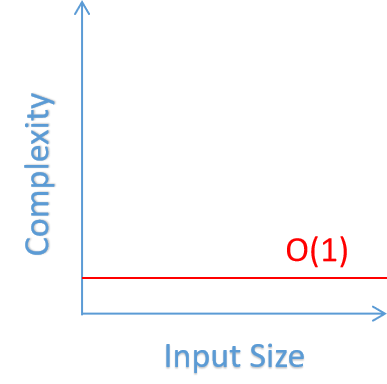
1. O(1) Constant runtime complexity #

This means that the algorithm does a fixed number of operations no matter the number of inputs.

Let's look at the code snippet below:

def first_element(array):
    print(array[0])

The function first_element() takes an array passed in and prints the first element and does not consider how many elements are present in the array.

Take a look at the graph representation below:

O(1) graph</br> Image Source

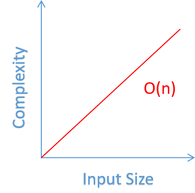
2. O(n) Linear runtime complexity #

This means that the runtime complexity of your algorithm increases linearly with the size of the input data.

Example:

def show_array_elements(array):
    for i in range(len(array)):   
        print(array[i]+"\n")

The code takes in an array using the function show_array_elements() and displays the array elements. If the array passed in as an argument only has 1 element, then the algorithm will only take 1 operation to run and would similarly take 300 operations for an array with 300 elements. The number of times the loop iterates depends on the number of array elements.

O(n) graph</br> Image Source</br>

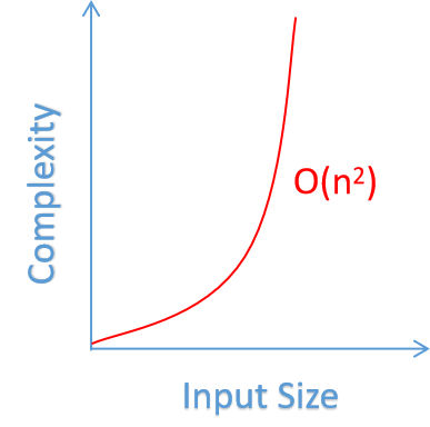
3. O(n²) Quadratic runtime complexity #

The algorithm varies with the square of the problem size, n.

Example:

def add_array_elements(array):  

    sum = 0  
    for i in range(len(array)):      
        for j in range (len(array)):         
            sum += array[i]+array[j] 
         
    return sum

The code has two loops, the outer, and the inner. The outer loop iterates n times giving an element to the inner loop which again loops n times, per one loop of the outer array, adding the element given by the outer array and all the array elements.

Taking a case where the array has 3 elements; the outer loop takes 3 operations in total to iterate over each element. For every 3 operations of the outer loop, the inner loop also takes 3 operations to iterate over each element. That is 3 × 3 operations amounting to 9.

O(n²) graph</br> Image Source</br>

4. O(log₂n)- Logarithmic runtime complexity #

This is associated with the binary search algorithm that searches by doing necessary halvings to get the item being searched for. The essence of this method is to compare the value being searched for, let's name it X, with the middle element of the array and if X is not found there.

We then decide which half of the array to look at next, which is repeated until X is found. The expected number of steps depends on the number of halvings needed to get from n elements to 1 element.

Have a look at the code and graphical illustrations below:

def binary_search(array, query):
    lower_bound = 0
    upper_bound = len(array)-1
    found_bool = False
    while (lower_bound <= upper_bound and found_bool == False):

        middle_value = (lower_bound + upper_bound) // 2
        
        if array[middle_value] == query:
           found_bool = True
           return found_bool

        elif query > array[middle_value]:
           lower_bound = middle_value + 1 
           
        else:
           upper_bound = middle_value - 1
           
    return found_bool

array = [1,2,3,4,5,6,7,8,9]
query = 7

val_found = binary_search(array, query)

Step 1 The code takes in a sorted array with 9 elements through the function binary_search() and searches for the value, the parameter named query, 7. It divides it in half and checks if 7 is in the middle.

1	2	3	4	5	6	7	8	9

Step 2 The middle value is 5 and our algorithm checks it with 7 and since 7 is greater than 5, then it will move to the right-hand side.

1	2	3	4	5	6	7	8	9

Step 3 We now have an array with 4 elements. The algorithm will divide it by half to get two arrays with 6 & 7 and 8 & 9. The one with 8 & 9 will be ignored and the algorithm will now check and compare 6 and 7.

1	2	3	4	5	6	7	8	9

Step 4 The comparison will be done and we will arrive at 7.

1	2	3	4	5	6	7	8	9

Further example inputs and the maximum number of steps to be taken are shown in the table below:

n	log<sub>2</sub>n
10	4
100	7
1000	10
10000	14
100000	17

O(log₂n) graph</br> Image Source

Determining the Big-O of an algorithm #

Here we look at the best-case and worst-case scenarios.</br>

Best and worst-case scenarios #

We will base our inferences based on the code below:

def linear_search(array, query):

    for i in range(len(array)):
        if array[i] == query:
            return i
    return -1

def binary_search(array, value):
    lower_bound = 0
    upper_bound = len(array)-1
    found_bool = False
    while (lower_bound <= upper_bound and found_bool == False):

        middle_value = (lower_bound + upper_bound) // 2
        
        if array[middle_value] == value:
           found_bool = True
           return found_bool
          
        elif value > array[middle_value]:
           lower_bound = middle_value + 1 
           
        else:
           upper_bound = middle_value - 1
           
    return found_bool

array = [1,2,3,4,5,6,7,8,9]
value = 7

The best case for linear_search() would be finding the value 1, O(1), while the worst case would be finding the last array element or a value not included in the array O(n). This is because it needs to traverse each element giving an O(n) complexity.

The best case for the binary_search() would be searching for the value of 5, which is the value in the middle of the array O(1). The worst-case would be searching the value 1 or 10, the first and the last elements of the array, or a value not included in the array. This is because the algorithm needs to make the halvings necessary until it reaches the first and the last elements (O(log₂n)).

Checking the Big O of a sample code #

We will look at the worst-case scenario perspective.

We will estimate the Big O of the code below (we are simply estimating its complexity, no conditional checks have been put for the code):

def array_arithmetic(array):
    
    value = 0  # O(1) complexity

    for e in range(len(array)): # O(n) complexity

        for j in range(10): # O(10) complexity
        
            for k in range(len(array)//2): # O(n/2) complexity
                
                value += array[e] + array[j] + array[k] # O(1) complexity
           
    return value # O(1) complexity

We should start with the innermost loop.

1. The innermost loop has O(n/2) complexity while its operation has O(1) complexity. The innermost loop therefore has (n/2) * (1) complexity.

2. The second inner loop has O(10) complexity and the inner loop (in No. 1) of this loop has O(n/2) meaning the whole second inner loop has (10) * (n/2) = O(5n) complexity.

3. An outer loop has O(n) complexity. The inner loop (No. 2) of this outer loop has in total O(5n) complexity. So, they have n*5n = 5n² complexity.

4. Combining the loop's complexity together with the two operations outside the loop, we get 1+1+5n² = O(2+5n²).

We drop all constants when estimating the Big O notation in that we remain with O(n²) instead of O(2+5n²).

The code above therefore has O(n²) complexity.

That's all for now. Hope you will consider the scalability of your algorithm next time you write one.

Happy Coding!

---

Peer Review Contributions by: Saiharsha Balasubramaniam